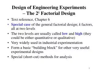
Design of Engineering Experiments – The 2 k Factorial Design

1. Design of Engineering Experiments– The 2k Factorial Design • Text reference, Chapter 6 • Special case of the general factorial design; k factors, all at two levels • The two levels are usually called low and high (they could be either quantitative or qualitative) • Very widely used in industrial experimentation • Form a basic “building block” for other very useful experimental designs • Special (short-cut) methods for analysis

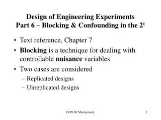
2. Design of Engineering Experiments– The 2k Factorial Design • Assumptions • The factors are fixed • The designs are completely randomized • Usual normality assumptions are satisfied • It provides the smallest number of runs can be studied in a complete factorial design – used as factor screening experiments • Linear response in the specified range is assumed

3. The Simplest Case: The 22 “-” and “+” denote the low and high levels of a factor, respectively Low and high are arbitrary terms Geometrically, the four runs form the corners of a square Factors can be quantitative or qualitative, although their treatment in the final model will be different

4. Chemical Process Example A = reactant concentration, B = catalyst amount, y = recovery

5. Analysis Procedure for a Factorial Design • Estimate factor effects • Formulate model • With replication, use full model • With an unreplicated design, use normal probability plots • Statistical testing (ANOVA) • Refine the model • Analyze residuals (graphical) • Interpret results

6. Estimation of Factor Effects See textbook, pg. 206 For manual calculations The effect estimates are: A = 8.33, B = -5.00, AB = 1.67 Practical interpretation

7. Estimation of Factor Effects • “(1), a, b, ab” – standard order • Used to determine the proper sign for each treatment combination

8. Statistical Testing - ANOVA Response:Conversion ANOVA for Selected Factorial ModelAnalysis of variance table [Partial sum of squares] Sum ofMeanFSourceSquaresDFSquareValueProb > F Model 291.67 3 97.22 24.82 0.0002A208.331208.3353.19< 0.0001B75.00175.0019.150.0024AB8.3318.332.130.1828 Pure Error 31.33 8 3.92 Cor Total 323.00 11 Std. Dev. 1.98 R-Squared 0.9030 Mean 27.50 Adj R-Squared 0.8666 C.V. 7.20 Pred R-Squared 0.7817 PRESS 70.50 Adeq Precision 11.669 The F-test for the “model” source is testing the significance of the overall model; that is, is either A, B, or AB or some combination of these effects important?

9. Estimation of Factor EffectsForm Tentative Model Term Effect SumSqr % Contribution Model Intercept Model A 8.33333 208.333 64.4995 Model B -5 75 23.2198 Model AB 1.66667 8.33333 2.57998 Error Lack Of Fit 0 0 Error P Error 31.3333

10. Regression Model y = bo + b1x1 + b2x2 + b12x1x2 + e or let x3 = x1x2, b3 = b12 y = bo + b1x1 + b2x2 + b3x3 + e A linear regression model. Coded variables are related to natural variables by Therefore,

11. Statistical Testing - ANOVA CoefficientStandard95% CI95% CI FactorEstimateDFErrorLowHighVIF Intercept 27.50 1 0.57 26.18 28.82 A-Concent 4.17 1 0.57 2.85 5.48 1.00 B-Catalyst -2.50 1 0.57 -3.82 -1.18 1.00 AB 0.83 1 0.57 -0.48 2.15 1.00 General formulas for the standard errors of the model coefficients and the confidence intervals are available. They will be given later.

12. Refined/reduced Model y = bo + b1x1 + b2x2 + e Response:Conversion ANOVA for Selected Factorial ModelAnalysis of variance table [Partial sum of squares] Sum ofMeanFSourceSquaresDFSquareValueProb > F Model 283.33 2 141.67 32.14 < 0.0001A208.331208.3347.27< 0.0001B75.00175.0017.020.0026 Residual 39.67 9 4.41Lack of Fit8.3318.332.130.1828Pure Error31.3383.92 Cor Total 323.00 11 Std. Dev. 2.10 R-Squared 0.8772 Mean 27.50 Adj R-Squared 0.8499 C.V. 7.63 Pred R-Squared 0.7817 PRESS 70.52 Adeq Precision 12.702 There is now a residual sum of squares, partitioned into a “lack of fit” component (the AB interaction) and a “pure error” component

13. Regression Model for the Process

14. Residuals and Diagnostic Checking

15. The Response Surface Direction of potential improvement for a process (method of steepest ascent)