Download
1 / 1
10 likes | 201 Vues
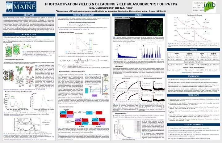
THE UNIVERSITY OF. 1 8 6 5. MAINE. B. A. Readout LASER ON 5s. Activation LASER OFF. Readout LASER OFF. Activation LASER ON 5s. Readout LASER ON 5s. Readout LASER OFF. Activation LASER OFF. Activation LASER ON 5s. 440. 460. 480. 500. 520. 540. 560. 580. 600. 250. 300.

E N D
THE UNIVERSITY OF 1 8 6 5 MAINE B A Readout LASER ON 5s Activation LASER OFF Readout LASER OFF Activation LASER ON 5s Readout LASER ON 5s Readout LASER OFF Activation LASER OFF Activation LASER ON 5s 440 460 480 500 520 540 560 580 600 250 300 350 400 450 500 550 600 Activation LASER OFF Activation LASER ON 2s D B A C Readout LASER ON 5s Readout LASER OFF τ =5.0 ± 0.4 τ =2.7 ± 0.3 τ =3.6 ± 0.4 τ =4.1 ± 0.4 Inactive State Active State λactivation λreadout λfluorescence B A Inverted type Microscope System Fig. 5. Experimental Geometry. Laser beams entering through the back of the objective to the sample. A lens is introduced to focus the beam to the focal plane of the objective hence spreading the beam at the sample which allows greater imaging area. Number of active molecules Na(t) Vs. Activation time t Readout Activation and Bleaching Photoactivation Sample Fitted A B B A Φra = (5.5 ± 0.2) x 10-7 Φb = (5.4 ± 0.1) x 10-6 Φra = (2.12 ± 0.02) x 10-6 Φb = (5.52 ± 0.03) x 10-6 Objective Lens Excitation Filter Φpa = (1.77 ± 0.02) x 10-6 Φpa = (1.10 ± 0.02) x 10-6 Dichroic Readout Laser D C D C (x104) C A B Emission Filter Φra = (7.1 ± 0.2) x 10-8 Φb = (1.85 ± 0.02) x 10-5 Φra = (2.28 ± 0.05) x 10-8 Φb = (5.76 ± 0.02) x 10-6 0.14 16 Photoactivation Laser 14 10 cycles CCD Camera Active 0.12 Inactive 12 0.1 Start Imaging Readout LASER OFF Readout LASER ON ~300s Φpa = (1.64 ± 0.07) x 10-5 Φpa = (1.19 ± 0.03) x 10-5 10 475 nm ex 0.08 Absorbance Fluorescence (cps) 8 0.06 Fig. 11. Experimental data fitted to Eq 1. Readout activation Yield and Bleaching Yield denoted as Φra and Φb respectively. (A)/(C) Experiment on PAGFP/wEosFP dried on a coverslip. (B)/(D) Experiment on PLL attached PAGFP/wEosFP in pH 7 buffer. 6 Fig. 10. Experimental data fitted to Eq 1. assuming no bleaching. Photoactivation Yield denoted as Φpa (A)/(C) Experiment on PAGFP/wEosFP dried on a coverslip. (B)/(D) Experiment on PLL attached PAGFP/wEosFP in pH 7 buffer. 0.04 4 0.02 2 End Imaging 0 0 Wavelength (nm) Wavelength (nm) Histogram Method 5 30 cycles 30 cycles By plotting the number of molecules in a given radius from a detected molecule in subsequent frames a Probability distribution histogram for detecting a molecule after a time lapse is generated. Using this histogram the area was calculated to get a relative magnitude of the total probability (Total number) of detecting a molecule in a subsequent frame. By plotting this area vs. the frame # and fitting it to an exponential decay model the decay time in terms of frames was found. Along with the average excitation rate per molecule in the region and the time per frame the bleaching yield was calculated. Absorbance/Fluorescence Bleaching Absorbance Excitation Emission Probability Density Fig 12.Distribution of the Probability Density Vs. the radial displacement for the dried EosFP sample.The colored lined shows the distribution for each consecutive frame from 0-10. 300 500 400 600 Wavelength (nm) Radial Displacement (μm) I N S T I T U T E F O R M O L E C U L A R B I O P H Y S I C S PHOTOACTIVATION YIELDS & BLEACHING YIELD MEASUREMENTS FOR PA FPs M.S. Gunewardene* and S.T. Hess* *Department of Physics & Astronomy and Institute for Molecular Biophysics, University of Maine, Orono, ME 04469. ANALYSIS ABSTRACT THEORY & METHODOLOGY Total Number Vs. Frame # Counting and Localizing Molecules6 Recent developments in single-molecule localization-based fluorescence methods are breaking the diffraction barrier of light microscopy. Hence a better understanding of photophysical parameters for cell-compatible photoactivatable/switchable fluorescent proteins (PA-FPs) is in demand. The Photoactivation yield (probability of activation of such a molecule upon receiving an activation photon), readout laser Photoactivation yield, and the photobleaching yield are important parameters of interest to optimize these microscopic techniques. A basic model for the dependence of the number of active molecules as a function of excitation time for two commonly used PA-FPs is derived using linear first-order kinetics. Single molecules were imaged by a high-sensitivity camera in a widefield fluorescence microscope under laser excitation. Analyzing measurements using the above model, the activation yields and the bleaching yield for PAGFP and Wild type EosFP were determined under different conditions. Here we present the data and compare results for each of the species. Practical implications of the measured yields will be discussed. The Photoactivation and Readout LASERs are used to control the number of active molecules in a sample at a given time. Hence the following two major processes are of interest . • Activation/Bleaching by Photoactivation Photons. • Activation/Bleaching by Readout Photons. we propose a photoconversion scheme 3 using linear first order kinetics given by the following figure. Ref: S.T.Hess et al, J. Phys. Chem. B 2004, 108, 10138-10148 Photoconversion Scheme INTRODUCTION Photo-Activatable Green Fluorescent Protein (PAGFP) The wild type of this protein is extracted from a Pacific Ocean jelly fish “Aequorea Victoria” The protein has 238 amino acids and the mutation at the amino acid site 203 Threonine with a Histidine (T203H) is known as PAGFP. Fig. 8. Molecule detection and localization procedure. (A) the raw image from the camera. (B) image after uniform background subtraction. (C) After setting upper and lower bound pixel thresholds to the uniform background subtracted image, green boxes - Localized molecules, red boxes - spot with insufficient number of lower threshold pixels. Fig 13. Total Number vs. frame # curves. The data points were fitted to y = A exp(-x/τ) + c model to determine the decay time. (A)-PAGFP dry, (B)-PAGFP in pH7 buffer, (A)-EosFP dry, (B)-EosFP in pH7 buffer. RESULTS Fig. 1. (A) β barrel structure of GFP. Has a diameter of ~30Å and a length of ~40 Å. (B)chemical structure of the chromophore also shown at the center in fig 1. A (yellow structure). Figure from: userpages.umbc.edu/~jili/ench772/intro.html Fig. 5. Common Photoconversion Scheme for PAGFP and wEosFP kdp and kpare the rate constants for ground state inter-conversions. Can show that the functional dependence of the active type molecules upon activation time is given by, Eos Fluorescent Protein (EosFP) The wild type of this protein (wEosFP) is extracted from a scleractinian coral Lobophyllia hemprichii and been named after the goddess of dawn Eos in Greek mythology. Fig. 9. Distribution of the number of active molecules in each frame at different stages of the experiment done on PAGFP dry sample. (A) the initial decay shows photobleaching of molecules due to the readout laser. (B) a section of the activation stage with 2s activations till frame ~2850 and 5s activations after frame ~2930. Each activation is followed by a readout . ------- Eq. 1 Where, k a / kb – Activation / Bleaching excitation rates per molecule. Φa / Φb - Activation / Bleaching Yields. n a / nn - Number of Active / Inactive type molecules, the 0 subscript denotes the initial numbers. Fig. 2. Molecular structure of EosFP. (A) Ribbon diagram of the EosFP tetramer. For one of the monomers, green and red colors indicate the protein fragments created by photoconversion. The atoms in the chromophore are color-coded. (B and C) The electron densities (2 Fo - Fc) of the green (B) and red (C) chromophores are contoured at 1.2 σ. (D and E) The hydrogen bonds constraining the green (D) and red (E) chromophores are represented by dashed lines. The dashed arrow depicts the interaction between the Glu-212 carboxyl and His-62 Cβ–H that is essential for cleavage of the His-62 Nα–Cα bond. Fitting Method From the data extracted from the above routine, the number of active molecules detected vs. the activation time graphs were plotted, The average excitation rate per molecule was calculated using the absorbance curves and an imaged laser profile for each fit. Hence a curve was fitted to the data to extract the yields. The photoactivation laser power at the sample was assumed low enough for little or no photobleaching. Experimental Setup and Sample Preparation Table 1. Summary of the measured Yields An Olympus IX71 inverted type microscope with NA 1.2 water immersed objective was used along with excitation filters Z496/10X/Z514/10X, emission filters ET525/50M/HQ590/75M, and beam splitters. The lasers were aligned to have the profiles centered. An Ar+ continuous-wave laser was used to generate the 496nm/514nm Readout Laser lines with ~10mW at the back of the objective and a 405nm semiconductor laser as the Activation Laser with ~2.5mW at the back of the objective (less power to have insignificant amount of photobleaching) were used to image PAGFP/wEosFP samples both dry as well as in Phosphate pH buffer. Protein samples were diluted and prepared at desired concentration to have a S/N ratio >10. A Photometrics Cascade 512 B CCD Camera was used for imaging with frame time set to 150ms with minimal delay time. CONCLUSIONS The wEosFP seems to be easily activated compared to PAGFP using 405nm photons. For PAGFP the Readout activation Yield and Photoactivation Yield were the same order of magnitude. Bleaching yields from the two methods were one order of magnitude different. The Fitting method seems less accurate since it uses small time scale fitting for evaluating the bleaching yield. The condition for same rate of Activation and Bleaching is, kaΦann(t)=kbΦbna(t). If an experiment is performed at this condition for sufficient enough time to gather the data, a single laser is sufficient for both the readout and activation processes. (demonstrated in Hess et al., 2007 and Hess et al. 2006) Figure from: Karin Nienhaus et al. (Jun 28, 2005) PNAS. vol. 102 no. 26, 9156–9159 Absorbance /Emission Spectral Characteristics REFERENCES The samples were prepared at room temperature and placed on 0.17mm thickness 22mm x 22mm coverslips for imaging. The samples were diluted using UV treated HPLC water. For experiments with buffer, coverslips were coated with Poly-L-Lysine (PLL) and the proteins were allowed to attach before the pH buffer solution was introduced. • Patterson, G.H et.al.. “A photoactivatable GFP for selective photolabeling of proteins and cells.” 2002 Science 297(5588): 1873-1877. • Wiedenmann, J et.al. “EosFP, a fluorescent marker protein with UV-inducible green-to-red fluorescence conversion.” 2004 PNAS 101: 15905-15910. • Hess, S.T. et al. “Fluorescence Photoconversion Kinetics in Novel Green Fluorescent Protein pH Sensors.” 2004 J. Phys. Chem. B 108: 10138-10148. • Lukyanov, K.A . et al. “Photoactivatable fluorescent proteins.” 2005(Nov.) Nat. Rev. Mol. cell Bio. 6: 885-891. • Hess, S.T. et al. “Dynamic clustered distribution of hemagglutinin resolved at 40nm in living cell membranes discriminates between raft theories.” 2007 PNAS 104: 17370-17375. • Hess, S.T. et al. “Ultra-High Resolution Imaging by Fluorescence Photoactivation Localization Microscopy.” 2006 Biophys. J.91 4258. ExperimentalProcedure Fig. 3. (A) Absorbance spectra. For PAGFP. Curve in Black/Green: Inactive/Active type (molecules before/after the illumination of UV radiation.) (B) Fluorescence spectrum at ~475nm excitation. Figure from: George H. Patterson, NIH ACKNOWLEDGEMENTS Dr. George Patterson at NIH for providing T203H mutant samples and spectral data. Dr.Uli Nienhaus and Dr.Jöerg Widenmann (University of Ulm) and Dr.Jöerg Bewersdorf (Jackson Lab, Bar Harbor) for the help in providing the wild-type EosFP samples.. Dr. Mike Mason at Chem. Eng. Dept. UMaine for the guidance and advice given on background signal reduction of solutions and coverslips for the experiment. Tom Tripp, Travis Gould, Ed Allgeyer of Dept. of Physics UMaine for technical support. Fig. 7. Experimental Procedure. The first 10 cycles are used to bleach off any background fluorescent molecules to a desirable level. Next, Imaging done for ~300s, the variation of active type molecules at this step will be used to find the Readout activation and Bleaching yields. The next activation cycles by the Photoactivation laser is used to determine the Photoactivation yield. Fig. 4. Spectra of the green and red states of EosFP at pH 7. (A) Green species. (B) Red species Excitation (emission) spectra were measured with emission (excitation) set to 520 (490) nm. ■: conversion yields scaled to the absorbance. (Inset) In vitro chromophore maturation at 27°C determined from the absorbance at 506 nm (solid line, exponential fit). Figure from: Jörg Wiedenmann et al. Nov 9, 2004 PNAS vol. 101 no. 45 15905–15910 Experiments were performed on the two fluorescent proteins, both dry and in pH 7 buffer. The captured images were later analyzed to count the number of active type molecules in each frame. Hence the idea is by getting the variation of such molecules with the activation time along with the theoretical model derived to calculate the yields.