Download

1 / 34
350 likes | 470 Vues
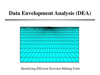
Data Envelopment Analysis: Introduction and an Application to University Administration By Emmanuel Thanassoulis, Professor in Management Sciences Aston University, Birmingham, UK E.thanassoulis@aston.ac.uk . Outline. Introduction to DEA: a graphical example

E N D
Data Envelopment Analysis: Introduction and an Application to University Administration ByEmmanuel Thanassoulis, Professor in Management Sciences Aston University, Birmingham, UK E.thanassoulis@aston.ac.uk
Outline • Introduction to DEA: a graphical example • DEA models: mathematical generalisation • An Application of DEA to University Administration
DMUs Inputs and Outputs • DEA: a method for comparing homogeneous operating units such as schools, hospitals, police forces, individuals etc on efficiency. Outputs The operating units typically produce or otherwise enable some useful outcomes (e.g. goods or services such as education or health outcomes) DMU Decision Making Unit Inputs The operating units typically use resources DEA makes it possible to compare the operating units on the levels of outputs they secure relative to their input levels.
Graphical Example on DEA • What is the efficiency of Hospital HO1 in terms of scope to reduce doctor andnurse numbers? Normalise inputs per 1000 outpatients
Deploy the Interpolation Principle to Create a set of Feasible ‘hospitals’ • We assume that interpolation of hospitals yields input output levels which are feasible in principle. • Example: take 0.5 of the input-output levels of hospital 2 and 0.5 of the input-output levels of hospital 3 and combine: 0.5 HO2 +0.5HO3 =
Feasible units (Hospitals) • The interpolation assumption means that 19 doctors and 33 nurses, though observed at no hospital, are capable of handling 1000 outpatients. Further, any hospital is also feasible if its input -output levels satisfy number of doctors 19. number of nurses 33 andoutpatients 1000.
Min θ Such that: A linear programming approach doctors:25l1+ 10 l2 + 28 l3 + 30 l4 + 40 l5 + 30 l6 nurses :60l1 + 50 l2 + 16 l3 + 40 l4 + 70 l5 + 50 l6 outpatients : 1000l1 + 1000 l2 + 1000 l3 + 1000 l4 + 1000 l5 + 1000 l6 l1, l2, l3,l4 ,l5, l6>= 0 . ≤ 25 θ ≤ 60 θ ≥1000 H02 and H03 are efficient peers to H01. Efficient Doctor-Nurse levels for H01 are (16.1, 38.5)
SAMPLE AREAS WHERE DEA HAS BEEN USED • Banking • Education • Regulation of ‘natural’ monopolies (e.g. water distribution, electricity, gas) • Tax collection • Courts • Sales forces (e.g. insurance sales teams)
TYPES OF ANALYSIS • Relative efficiency measure; • Identification of efficient exemplar units; • Target setting. • decomposing efficiency in layered data (pupil, school, type of school etc); • Decomposing productivity changes over time into those attributable to the unit and those to technology shift (Malmquist Indices) • Identifying the increasing/decreasing returns to scale; • Measuring scale elasticity; • Identifying most productive scale size;
ASSESSING EFFICIENCY AND PRODUCTIVITY IN UK UNIVERSITY ADMINISTRATION1999/00 TO 2004/05. Prof. Emmanuel Thanassoulis e.thanassoulis@aston.ac.uk
Aim of this project • To identify units with cost-efficient good quality administrative services and disseminate good practice; • To assess changes in the productivity of UK university administration over time (1999/00 to 2004/5).
Motivation for the Study • Expenditure on Administration and Central Services is about 20% of total HEI expenditure in the UK Hence expenditure on administration is substantial and competing with direct expenditure on academic activities.
Questions to be addressed: • Are efficiency savings possible? • Is there a trade-off between expenditure and quality of service in administration ? • Has there been any change over time in productivity of administrative services in UK Higher Education Institutions (HEIs)?
The Assessment Method We opted for Data Envelopment Analysis (DEA). This is a linear programming based benchmarking method. It identifies cost-efficient benchmark units and then assesses the scope for savings at the rest of the units relative to the benchmarks.
DEA is illustrated in the graph below. An ‘efficient boundary’is created from benchmark units (CAS12 and CAS2). Thevirtualbenchmark VBM6 offers the top levels of research grants and students when keeping to the mix of research grants to students of CAS6. VBM6 The distance from CAS6 to VBM6 reflects the scope for savings at CAS 6. Data Envelopment Analysis (DEA)
Unit of Assessment The unit of assessment includes core CAS and administration devolved away from the centre; It excludes Estates, Libraries, Residences and catering.
The Unit of Assessment Initial consultations with senior administrators and academics suggested the following conceptual framework for the unit of assessment: Support for students Support for non admin staff Support for research
Input – Output Set Assessments were carried out by setting the Admin costs against the Measures of Admin Volume shown (at university level).
Model Specification • VRS model – Input oriented • Outliers have been re-scaled to be on the boundary formed by the non-outlier units; • A balanced panel between the first (1999/00) and the last (2004/5) year is reported upon here. • 100 universities are therefore included in the assessment reported here.
Findings at University Level - illustration • The efficiency here is a percentage. It means the observed admin staff costs can be reduced each year to the percentage indicated above (e.g. 57.57% in 1999/00). • So relative to benchmark institutions for student income, non admin staff expenditure and research income, administrative staff costs could be about half. • The scope for efficiency savings on Operating Expenditure is less than for administrative staff, at about 25% - 30%. • If we assume Staff and OPEX can substitute for each other then the scope for efficiency savings is 30% or so on each one of administrative staff and OPEX. Efficiency Scores at a sample admin unit
Comparing the sample university with its benchmark units on Administrative Staff Costs • Data is indexed so that sample university of the previous slide = 1 on each variable.
Sector Findings on Efficiency • There are some 20 units with good benchmark performance without any scope for further efficiency savings. About half of these benchmark units are found to be consistently cost-efficient in all six years of our analysis. These units could prove examples of good operating practices in administration. • On the other hand some of the units with large scope for efficiency savings are so on all the six years suggesting persistent issues of expenditure control. • Visits to specific institutions did not support the notion that factors outside the model such as quality of service could explain differences in efficiency. • When we take administrative staff and OPEX as substitutable we find that the scope for efficiency savings is about 15% per annum in each.
Productivity is defined as the ratio of output to resource used. Assessing Productivity Change Over Time ]
Productivity change = Efficiency catch up x Boundary shift. / • Efficiency catch up ] • { X • }0.5 • Boundary shift
Bottom two HEIs on productivity Data for 2004/5 – constant prices, Normalised so that 1999/00 = 1 In both universities the normalised data show substantial rise in admin staff costs against modest rise or even drop in activities.
Top three HEIs on productivity Data for 2004/5 – constant prices, Normalisedso that1999/00 = 1 In these three universities that gain the most in admin productivity, admin costs fall over time while outputs rise, with only two exceptions on research income.
Productivity Change 1999/00 to 2004/5 – Staff Costs Model Deteriorating Improving NB: An index of 1 means stable productivity between 1999/0 and 2004/5. An index below 1 means productivity drop. Eg. a value of 0.9 means the same work load is costing in 2004/5 11% more than it did in 1999/0. An index above 1 means productivity improvement.
Productivity Change Decomposition – Staff Model • Benchmark performance tends to deteriorate over time. • HEIs tend to catch up with the boundary over time. Efficiency Catch-up Boundary Shift • HEIs with negative effects due to scale exceed those with positive effects Scale Efficiency Catch-up
Productivity Change 1999/00 to 2004/5 – Staff and OPEX Combined Deteriorating Improving • We have a virtually symmetrical distribution with half the units improving and the rest deteriorating in productivity.
Productivity Change Decomposition – Joint Model • There is clear evidence that the boundary is improving in that best performance is more productive in 2004/5 than in 1999/0. Most units are falling behind the boundary. Efficiency Catch-up Boundary Shift • The catch-up and boundary shift results are the reverse from when staff costs were the sole input. This suggests perhaps that non staff expenses were managed better than staff costs, over time. • Scale efficiency deteriorates over time. Scale Efficiency Catch-up
Summary of Findings on Productivity at Sector Level • Between 1999/00 and 2004/5 we find a divergent picture between administrative staff cost on the one hand and OPEX or the two inputs taken jointly on the other. In the case of administrative staff taken as the sole input we find that there is on average a drop in productivity so that for given levels of the proxy output variables staff cost is about 95% in 1999/00 compared to what it is in 2004/5, at constant prices. • Looking deeper it is found that generally units do keep up with the benchmark units but it is the benchmark units that are performing less productively by almost 7% in 2004/5 compared to 1999/00. The situation is not helped by a slight loss of productivity through scale sizes becoming less productive, by about 1.5% in 2004/5 compared to 1999/00. • In contrast when we look at OPEX as a sole input or indeed at administrative staff and OPEX as joint resources we find that productivity is more or less stable between 1999/00 and 2004/5. There is a slight loss of about 2% but given the noise in the data this is not significant.
What is significantly different between administrative staff on the one hand and OPEX or the two joint inputs on the other is that benchmark performance improves on average by about 8% between 1999/00 and 2004/5. • Unfortunately non benchmark units cannot quite keep up with this higher productivity. Also there is a slight deterioration again in scale size efficiency and the net effect is that despite the improved benchmark productivity, productivity on average is stable to slightly down between 1999/00 and 2004/5. • As with cost efficient practices here too our analysis has identified a small set of units which register significant productivity gains and others which register significant productivity losses between 1999/00 and 2004/5. An investigation of the causes in each case would be instrumental for offering advice to other units on how to gain in productivity over time and avoid losses.