Postdocs , Students:
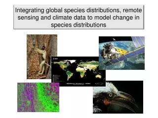
Integrating global species distributions, remote sensing and climate data to model change in species distributions. Integrating global species distributions, remote sensing and climate data to model change in species distributions.

Postdocs , Students:
E N D
Presentation Transcript
Integrating global species distributions, remote sensing and climate data to model change in species distributions
Integrating global species distributions, remote sensing and climate data to model change in species distributions Walter Jetz (Yale U), Rob Guralnick (CU Boulder, Brian McGill (U Maine), Rama Nemani (NASA Ames), Forrest Melton (NASA Ames) PIs: Dr. Mao-Ning Tuanmu (Yale U, NASA-funded), Dr. Adam Wilson (Yale U, YCEI-funded), Dr. Benoit Parmentier (NCEAS, iPlant-funded), Natalie Robinson (CU Boulder, NASA-funded), George Cooper (U Maine, NASA-funded) Postdocs, Students: Dr. Jim Regetz (NCEAS), Dr. Mark Schildhauer (NCEAS), Martha Narro (iPlant), Dave Thau (Google), Jeremy Malczyk (Yale U) Others: YCEI
Hierarchical Bayesian models Global 1km environmental layers Models Predictions Inference • Environment • Topography: 90m global DEM • Land cover type: Consensus • Habitat Heterogeneity • Net primary productivity • Climate • Temperature: in progress • Cloud cover: close! • Precipitation: in progress • Bioclimatic variables • Extreme events Global spatial biodiversity data Quality Control Map of Life Change in: Species niches Species distributions 1972-92 vs. 1992-12
Amphibians Mammals GBIF record count GBIF species richness Expert species richness Meyer, Guralnick, Kreft & Jetz in prep.
Spatial biodiversity data Hurlbert and Jetz (PNAS 2007) Jetz et al. (Conservation Biology 2008)
Map of Life - An infrastructure for integrating and analyzing global species distribution knowledge mappinglife.org Jetz et al. 2012, TREE
Map of Life • An online workbench and knowledgebase to dynamically document, integrate, validate, advance, analyze the disparate sources of global biodiversity distribution knowledge • Tools and products: • Aquatic and terrestrial global biodiversity layers • Species lists for user-defined regions, on mobile devices • Dynamically-updated threat assessments Jetz et al. 2012, TREE
1. Full global-extent 90m DEM ASTER GDEM V2 Blended, void-filled, multi-scale smoothed SRTM V4 For global derivation of terrain variables and distribution modeling Robinson et al (MS)
2. Global consensus land cover Limitations of Existing Products • Classification errors • Among-product disagreements IGBP DISCover, U of Maryland, GLC2000 and MODIS; Herold et al. 2008
2. Global consensus land cover Limitations of Existing Products • Classification errors • Among-product disagreements • Categorical data – False absences of minor land cover classes
2. Global consensus land cover Goal Generate a harmonized set of 1-km resolution land cover product that provides scale-integrated and accuracy-weighted consensus land cover information on a continuous scale. Example use in biodiversity modeling: Minimize false absences and improve accuracy of species distribution models
2. Global consensus land cover 1km Land Cover Prevalence
2. Global consensus land cover Improvements to model accuracy Better Tuanmu & Jetz (Global Ecology & Biogeography, in review)
3. Global temp. & prec. layers Satellite-Station Data Fusion Climate-aided interpolation Monthly climatologies (2000-2011) from MODIS and station means Interpolate daily station anomalies (including pre 2000) Goal: Develop daily 1km surfaces of tmax, tmin, and ppt with MODIS and climate station data (1970-2011).
3. Global temp. & prec. layers Satellite Weather Products Temperature: MODIS LST (MOD11A1) Precipitation:MODIS Cloud Product (MOD06)
3. Global temp. & prec. layers CLIMATE INTERPOLATION WORKFLOW All the steps are implemented in Open Source GIS combining Linux Shell script, PostGres, R, Python, GRASS and GDAL.
3. Global temp. & prec. layers Temperature (deg Celsius) Max. temperature, 1 Sep. 2010 Climate aided interpolation Comparison of models
3. Global temp. & prec. layers MOD35 Cloud Frequency (%) in February Venezuela (MODIS tile h11v08)
3. Global temp. & prec. layers MOD35 Cloud Frequency (%) in February
3. Global temp. & prec. layers Cloud data improves interpolation accuracy
3. Global temp. & prec. layers Comparison of WorldClim and MOD35-informed mean monthly interpolation (February) mm Worldclim MOD35-Informed Mean monthly precipitation (mm) from WorldClim [lppt~s(y,x)+s(dem)] and MOD35-informed interpolation[lppt~s(y,x)+s(dem)+cld+cot+cer20 ]
LandcoverBias in Collection 5 (MOD35) Cloud Data 100 MOD35 Collection 5 MOD35 Collection 6 80 Non-Forest 60 40 20 0 Cloud Frequency (%) in March • The current (C5) MODIS Cloud mask has more frequent “cloudy” days over non-forest • The updated (C6) mask less biased by land cover
Range Refinement 180,000km2 Expert range size: 180,000km2 23,000km2 MODIS Landcover 2001-2012 Expert range Suitable 2012 Hartlaub’sTuraco: forest specialist, >1500m elevation