Random-Packing Dynamics in Granular Flow
Random-Packing Dynamics in Granular Flow. Martin Z. Bazant Department of Mathematics, MIT. The Dry Fluids Laboratory @ MIT Students: Chris Rycroft, Ken Karmin, Jeremie Palacci, Jaehyuk Choi (PhD ‘05) Collaborators: Arshad Kudrolli (Clark University, Physics)

Random-Packing Dynamics in Granular Flow
E N D
Presentation Transcript
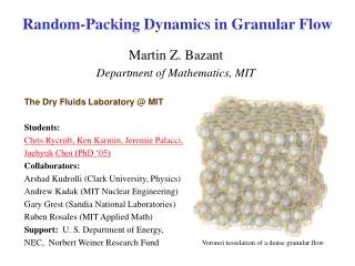
Random-Packing Dynamics in Granular Flow Martin Z. Bazant Department of Mathematics, MIT The Dry Fluids Laboratory @ MIT Students: Chris Rycroft, Ken Karmin, Jeremie Palacci, Jaehyuk Choi (PhD ‘05) Collaborators: Arshad Kudrolli (Clark University, Physics) Andrew Kadak (MIT Nuclear Engineering) Gary Grest (Sandia National Laboratories) Ruben Rosales (MIT Applied Math) Support: U. S. Department of Energy, NEC, Norbert Weiner Research Fund Voronoi tesselation of a dense granular flow
MIT Modular Pebble-Bed Reactor http://web.mit.edu/pebble-bed • Reactor Core : • D = 3.5 m • H = 8-10m • 100,000 pebbles • d = 6 cm • Q =1 pebble/min MIT Technology Review (2001)
Experiments and Simulations MIT Dry Fluids Lab http://math.mit.edu/dryfluids Half-Reactor Model (“coke bottle”) Kadak & Bazant (2004) Plastic or glass beads 3d Full-Scale Discrete- Element Simulations (“molecular dynamics”) Rycroft, Bazant, Landry, Grest (2005) Sandia parallel code from Gary Grest Frictional, visco-elastic spheres N=400,000 Quasi-2d Silo Experiments Choi et al., Phys. Rev. Lett. (2003) Choi et al., J. Phys. A: Condens. Mat. (2005) d=3mm glass beads Digital-video particle tracking near wall
How does a dense random packing flow? • Dilute random “packing” (gas) • Boltzmann’s kinetic theory: sudden randomizing collisions • Dense, ordered packing (crystal) • Vacancy/interstitial diffusion • Dislocations and other defects • Dense, random packing (liquid, glass, granular,...) • Long-lasting, many-body contacts • Are there any “defects”? • How to describe cooperative random motion?
L = 20cm D=2.5cm vz H=1m d=3mm z y x W Experimental Apparatus Dry Fluids Lab (MIT Applied Math) • Quasi-2D silo • W,D,L can be varied • t= 1ms (1000 frames/s) • Diffusion and mixing • is studied in nearly uniform flow • W: 8, 12, 16, …, 32 mm • vz (W-d)1.5 • Image processing:centeroid technique(d=15 pixels, x~0.003d)
NormalDiffusion SuperDiffusion NormalDiffusion SuperDiffusion Universal Crossover in Diffusion J. Choi, A. Kudrolli, R. R. Rosales, M. Z. Bazant, Phys. Rev. Lett. (2003). • x2t: = 1.5 1.0 • z2t : = 1.6 1.0 • Super-diffusion for z << d, • Diffusion for z >> d • Data collapses for all flowrates as a function ofdistance dropped (not time) • Suggests that fluctuationshave the same physicalorigin as the mean flow(not internal “temperature”)
u v v + dv The Mean Velocity in Silo Drainage Kinematic Model Choi, Kudrolli & Bazant, J. Phys. A: Condensed Matter (2005). Nedderman & Tuzun, Powder Tech. (1979) Diffusion equation… Green function = point opening Parabolic streamlines …but what is diffusing?
“The Paradox of Granular Diffusion” Particles diffuse much more slowly than free volume. Experiment by A. Samadani & A. Kudrolli (3mm glass beads)
Microscopic Flow Mechanisms for Dense Amorphous Materials 1. “Vacancy” mechanism for flow in viscous liquids (Eyring, 1936); Also: “free volume” theories of glasses (Turnbull & Cohen 1958, Spaepen 1977,…) 2. “Void” model for granular drainage (Litwiniszyn 1963, Mullins 1972) 3. “Spot” model for random-packing dynamics (M. Z. Bazant, Mechanics of Materials 2005) 4. “Localized inelastic transformations” (Argon 1979, Bulatov & Argon 1994) “Shear Transformation Zones” (Falk & Langer 1998, Lemaitre 2003)
Correlations Reduce Diffusion Simplest example: A uniform spot affects N particles. • Volume conservation (approx.) • Particle diffusion length Experiment: 0.0025 DEM Simulation: 0.0024 (some spot overlap)
Direct Evidence for Spots Spatial correlations in velocity fluctuations (like “dynamic hetrogeneity” in glasses) EXPERIMENTS SIMULATIONS • MIT Dry Fluids Lab • 3mm glass beads, slow flow (mm/sec) • particle tracking by digital video (at wall) • 125 frames/sec, 1024x1024 pixels • 0.01d displacements • Discrete-element method (DEM), spheres • Sandia parallel code on 32-96 processors • Friction, Coulomb yield criterion • Visco-elastic damping • Hertzian or Hookean contacts
DEM Spot Model Void Model Simple spot model predicts mean flow and tracer diffusion in silo drainage fairly well (with only 3 params), but does not enforce packing constraints. Simulations by Chris Rycroft
“Multi-scale” Spot Algorithm1. Simple spot-induced motion • Apply the usual spot displacement first to all particles within range
“Multi-scale” Spot Algorithm2. Relaxation by soft-core repulsion • Apply a relaxation step to all particles within a larger radius • All overlapping pairs of particles experience a normal repulsive displacement (soft-core elastic repulsion) • Very simple model - no “physical” parameters, only geometry.
“Multi-scale” Spot Algorithm3. Net cooperative displacement • Mean displacements are mostly determined by basic spot motion (80%), but packing constraints are also enforced • Can this algorithm preserve reasonable random packings? • Will it preserve the simple analytical features of the model?
Multiscale Spot Algorithm in Two Dimensions • Very strong tendency for crystal order • (Artificial) flow by dislocations, grain boundaries, similar to crystals • Fundamentally different from 3d…
Spot Model DEM Multiscale Spot Model In Three Dimensions Rycroft, Bazant, Grest, Landry (2005) • Infer 3 spot parameters from DEM, as from expts: * radius = 2.6 d * volume = 0.33 v * diffusion length = 1.39 d • Relax particles each step with soft-core repulsion • “Time” = number of drained particles • Very similar results as DEM, but >100x faster!
Spot Model vs. DEM: Mean velocity profile Excellent fit near bottom, but upper flow is more plug-like in MD. (Only one parameter, b, was fitted.)
Spot Model vs. DEM: Particle Diffusion Diffusive regime Superdiffusive regime • Relaxation only slightly enhances diffusion (spot-induced rearrangements) • Short-range (z<d) super-diffusion is not reproduced by the Spot Model.
Spot Model vs. DEM: Velocity correlations Very similar structure of dynamical correlations. (Only the decay length was fitted.)
Spot Model vs. DEM: “bond lengths” g(r) t = 1.0-1.4 sec Identical flowing structure, different from the initial condition, after substantial drainage has occurred. (Steady state?)
Spot Model vs. DEM: “bond angles” t = 1.0-1.4 sec Nearly identical flowing structure, different from the initial condition. Universal features of dense flowing hard spheres?
Universal Flowing States in Spot Simulations Taller Silos, more particles, longer drainage times g(r) • Reaches statistical steady state • Spot algorithm never breaks down • Some local ordering compared to DEM (involving only 1% of particles) • Seems to “converge” to DEM state (no ordering) as spot step size decreases • Largely insensitive to other parameters DEM flowing state Spot t = 8 sec Spot t = 16 sec 2. Periodic boundary conditions, unbiased spot diffusion (“glass”) • Also reaches statistical steady state • “Universal” for fixed volume fraction (independent of initial conditions, mostly insensitive to parameters) • New simulation method for (nearly) hard sphere systems
A Mathematical Theory of Spot-Induced Particle Motion Bazant, Mechanics of Materials (2005) Spot influence function A non-local stochastic differential equation for tracer diffusion: Interpret as the limit of a random (Riemann) sum of random variables:
Mean-Field Approximation (for spots) • Assume: • Poisson process for spot positions with (given) mean • Independent spot displacements Fokker-Planck equation Fluid velocity (opposes spot drift + climbs gradient in spot density) Diffusivity tensor In this way, particle flow and diffusion are expressed entirely in terms of spot dynamics, which must be derived from mechanical principles for a given material and geometry...
Classical Mohr-Coulomb Plasticity • 1. Theory of Static Stress in a Granular Material Assume “incipient yield” everywhere: • (t/s)max = m m= internal friction coefficient • = internal failure angle = tan-1m e = p/4-f/2 2. Theory of Plastic Flow (only in a wedge hopper!) Levy flow rule / Principle of coaxiality: Assume equal, continuous slip along both incipient yield planes (stress and strain-rate tensors have same eigenvectors)
Failures of Classical Mohr-Coulomb Plasticity to Describe Granular Flow 1. Stresses must change from active to passive at the onset of flow in a silo (to preserve coaxiality). Free surface “Active” (gravity-driven stress) Silo bottom “Passive” (side-wall-driven flow) Exit 2. Walls produce complicated velocity and stress discontinuities (“shocks”) not seen in experiments with cohesionless grains. 3. No dynamic friction 4. No discreteness and randomness in a “continuum element”
Idea (Ken Kamrin): Replace coaxiality with an appropriate discrete spot mechanism d Slip lines 2 Spot Stochastic “Flow Rule” D Spots random walk along Mohr-Coloumb slip lines (but not on a lattice) Similar ideas in lattice models for glasses: Bulatov and Argon (1993), Garrahan & Chandler (2004)
A Simple Theory of Spot Drift Spot = localized failure where is replaced by k (static to dynamic friction) (Assume quasi-static global mean stress distribution is unaffected by spots.) Net force on the particles affected by a spot A spot’s random walk is biased by this force projected along slip lines. Use the resulting spot drift and diffusivity in the general theory to obtain the fluid velocity and particle diffusivity…
Towards a General Theory of Dense Granular Flow? Gravity-driven drainage from a wide quasi-2d silo: Predicts the kinematic model Slip lines and spot drift vectors Mean velocity profile Coette cell with a rotating rough inner wall: Predicts shear localization
Spot Model DEM Trouble in Paradise? Particle Voronoi Volumes Chris Rycroft, PhD thesis • “Free volume” peaks in regions of highest shear, not the center! • Maybe somehow alter spot dynamics, or don’t use spots everywhere…
General Theory of Dense Granular Materials: Stochastic Elastoplasticity? • When forcing is first applied, the granular material responds like an elastic solid. • Whenever the stability criterion is violated, a plastic “liquid” region at incipient yield is born. • Stresses in elastic solid and plastic liquid regions evolve under load, separated by free boundaries. • Solid regions remain stagnant, while liquid regions flow by stochastic plasticity. Microscopic packing dynamics is described by the Spot Model. Classical engineering picture of silo flow with multiple zones, without any quantitative theory. (Nedderman 1991)
Conclusion • The Spot Model is a simple, general, and realistic mechanism for the dynamics of dense random packings • Random walk of spots along slip lines yields a Stochastic Flow Rule for continuum plasticity • Stochastic Mohr-Coulomb plasticity (+ nonlinear elasticity?) could be a general model for dense granular flow • Interactions between spots? Extend to 3d, other materials,…? For papers, talks, movies,… http://math.mit.edu/dryfluids
Mohr-Coulomb Stress Equations (assuming incipient yield everywhere) Characteristics (the slip-lines) e = p/4-f/2
Spot drift opposes the net material force. • Spots drift through slip-line field constrained only by the geometry of the slip-lines. Probability of motion along a slip-line is proportional to the component of –Fnet in that direction. Yields drift vector: • For diffusion coefficient D2, must solve for the unique probability distribution over the four possible steps which generates the drift vector and has forward and backward drift aligned with the drift direction. D1