Stochastic Context Free Grammars

1. Stochastic Context Free Grammars for noncoding RNA gene prediction CBB 261 B. Majoros

2. Formal Languages A formal language is simply a set of strings (i.e., sequences). That set may be infinite. Let M be a model denoting a language. If M is a generative model such as an HMM or a grammar, then L(M) denotes the language generated by M. If M is an acceptor model such as a finite automaton, then L(M) denotes the language accepted by M. When all the parameters of a stochastic generative model are known, we can ask: “What is the probability that model M will generate string S?” which we denote: P(S | M)

3. Recall: The Chomsky Hierarchy all languages Turing machines recursively enumerable languages recursive languages Halting TM’s Linear-bounded TM’s context sensitive languages SCFG’s / PDA’s context free languages regular languages HMM’s / reg. exp.’s * each class is a subset of the next higher class in the hierarchy Examples: * HMM-based gene-finders assume DNA is regular * secondary structure prediction assumes RNA is context-free * RNA pseudoknots are context-sensitive

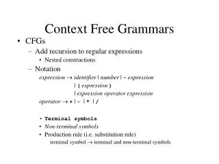
4. Context-free Grammars (CFG’s) A context-free grammar is a generative model denoted by a 4-tuple: G= (V, , S, R) where:  is a terminal alphabet, (e.g., {a, c, g, t} ) V is a nonterminal alphabet, (e.g., {A, B, C, D, E, ...} ) SV is a special start symbol, and R is a set of rewriting rules called productions. Productions in R are rules of the form: X→ for XV, (V)*; such a production denotes that the nonterminal symbol X may be rewritten by the expression , which may consist of zero or more terminals and nonterminals.

5. A Simple Example As an example, consider G=(VG, , S, RG), for VG={S, L, N}, ={a,c,g,t}, and RG the set consisting of: One possible derivation using this grammar is: S aSt acSgt acgScgt acgtSacgt acgtLacgt acgtNNNNacgt acgtaNNNacgt acgtacNNacgt acgtacgNacgt acgtacgtacgt S→aSt S→tSa S→cSg S→gSc S→L L→N N N N N→a|c|g|t S→aSt S→cSg S→gSc S→tSa S→L L→N N N N N→a N→c N→g N→t

6. Derivations Suppose a CFG G has generated a terminal stringx*. A derivation denotes a single way by which G may have generated x. For a grammar G and a string x, there may exist multiple distinct derivations. A derivation (or parse) consists of a series of applications of productions from R, beginning with the start symbolS and ending with a terminal stringx: Ss1s2s3Lx We can denote this more compactly as: S*x. Each string si in a derivation is called a sentential form, and may consist of both terminal and nonterminal symbols: si(V)*. Each step in a derivation must be of the form: wXzwz for w,z(V)*, where X→ is a production in R; note that w and z may be empty ( denotes the empty string).

7. Leftmost Derivations A leftmost derivation is one in which at each step the leftmost nonterminal in the current sentential form is the one which is rewritten: S LabXdYZabxxxdYZabxxxdyyyZabxxxyzdyyyzzz For many applications, it is not necessary to restrict one’s attention to only the leftmost derivations. In that case, there may exist multiple derivations which can produce the same exact string. However, when we get to stochastic CFG’s, it will be convenient to assume that only leftmost derivations are valid. This will simplify probability computations, since we don’t have to model the process of stochastically choosing a nonterminal to rewrite. Note that doing this does not reduce the representational power of the CFG in any way; it just makes it easier to work with.

8. Context-freeness The “context-freeness” of context-free grammars is imposed by the requirement that the l.h.s of each production rule may contain only a single symbol, and that symbol must be a nonterminal: X→ for XV, (V)*. That is, X is a nonterminal and  is any (possibly empty) string of terminals and/or nonterminals. Thus, a CFG cannot specify context-sensitive rules such as: wXz→wz which states that nonterminal X can be rewritten by  only when X occurs in the local context wXz in a sentential form. Such productions are possible in context-sensitive grammars (CSG’s).

9. Context-free Versus Regular The advantage of CFG’s over HMM’s lies in their ability to model arbitrary runs of matching pairs of “palindromic” elements, such as nested pairs of parentheses: L((((((((L))))))))L where each opening parenthesis must have exactly one matching closing parenthesis on the right. When the number of nested pairs is unbounded (i.e., a matching close parenthesis can be arbitrarily far away from its open parenthesis), a finite-state model such as a DFA or an HMM is inadequate to enforce the constraint that all left elements must have a matching right element. In contrast, the modeling of nested pairs of elements can be readily achieved in a CFG using rules such as X→(X). A sample derivation using such a rule is: X  (X)  ((X))  (((X)))  ((((X))))  (((((X))))) An additional rule such as X→is necessary to terminate the recursion.

10. Limitations of CFG’s One thing that CFG’s can’t model is the matching of arbitrary runs of matching elements in the same direction (i.e., not palindromic): ......abcdefg.......abcdefg..... In other words, languages of the form: wxw for strings w and x of arbitrary length, cannot be modeled using a CFG. More relevant to ncRNA prediction is the case of pseudoknots, which also cannot be recognized using standard CFG’s: ....abcde....rstuv.....edcba.....vutsr.... The problem is that the matching palindromes (and the regions separating them) are of arbitrary length. Q: why isn’t this very relevant to RNA structure prediction? Hint: think of the directionality of paired strands.

11. Stochastic CFG’s (SCFG’s) A stochastic context-free grammar (SCFG) is a CFG plus a probability distribution on productions: G= (V, , S, R, Pp) where Pp : R a¡, and probabilities are normalized at the level of each l.h.s. symbol X: [Pp(X→)=1 ] XVX→ Thus, we can compute the probability of a single derivation S*x by multiplying the probabilities for all productions used in the derivation: iP(Xi→i) We can sum over all possible (leftmost) derivations of a given string x to get the probability that G will generate x at random: P(x | G) =  P(Sj*x | G). j

12. A Simple Example As an example, consider G=(VG, , S, RG, PG), for VG={S, L, N}, ={a,c,g,t}, and RG the set consisting of: S→aSt|tSa|cSg|gSc|L L→N N N N N→a|c|g|t where PG(S→)=0.2, PG(L→NNNN)=1, and PG(N→)=0.25. Then the probability of the sequence acgtacgtacgt is given by: P(acgtacgtacgt) = P( SaStacSgtacgScgtacgtSacgt acgtLacgtacgtNNNNacgtacgtaNNNacgt acgtacNNacgtacgtacgNacgtacgtacgtacgt) = 0.2 × 0.2 × 0.2 × 0.2 × 0.2 × 1 × 0.25 × 0.25 × 0.25 × 0.25 = 1.25×10-6 because this sequence has only one possible leftmost derivation under grammar G. If multiple derivations were possible, we would use the Inside Algorithm. (P=0.2) (P=1.0) (P=0.25)

13. Implementing Zuker in an SCFG stems, bulges, internal loops i pairs with j loops multiloops i is unpaired j is unpaired i+1 pairs with j-1 Rivas & Eddy 2000 (Bioinformatics 16:583-605) . . .

14. Implementing Zuker in an SCFG Rivas & Eddy 2000 (Bioinformatics 16:583-605)

15. The Parsing Problem Two questions for a CFG: Can a grammar G derive string x? If so, what series of productions would be used during the derivation? (there may be multiple answers!) Additional questions for an SCFG: What is the probability that G derives string x? What is the most probable derivation of x via G? (likelihood)

16. Chomsky Normal Form (CNF) • Any CFG which does not derive the empty string (i.e.,   L(G)) can be converted into an equivalent grammar in Chomsky Normal Form (CNF). A CNF grammar is one in which all productions are of the form: • X→YZ • or: • X→a • for nonterminals X, Y, Z, and terminal a. • Transforming a CFG into CNF can be accomplished by appropriately-ordered application of the following operations: • eliminating useless symbols (nonterminals that only derive ) • eliminating null productions (X→) • eliminating unit productions (X→Y) • factoring long rhs expressions (A→abc factored into A→aB, B→bC, C→c) • factoring terminals (A→cB is factored into A→CB, C→c) • (see, e.g., Hopcroft & Ullman, 1979).

17. CNF - Example CNF: S→A ST|T SA|C SG|G SC|N L1 SA→S A ST→S T SC→S C SG→S G L1→NL2 L2→NN N→a|c|g|t A→a C→c G→g T→t Non-CNF: S→aSt|tSa|cSg|gSc|L L→N N N N N→a|c|g|t Disadvantages of CNF: (1) more nonterminals & productions, (2) more convoluted relation to problem domain (can be important when implementing posterior decoding) Advantages: (1) easy implementation of inference algorithms

18. The CYK Parsing Algorithm Cell (i, j) contains all the nonterminals X which can derive the entire subsequence: actagctatctagcttacggtaatcgcatcgcgc. (k+1, j) contains only those nonterminals which can derive the red substring. (i, k) contains only those nonterminals which can derive the green substring. j C k (k+1, j) atcgatcgatcgtagccctatccctagctatctagcttacggtaatcgcatcgcgcgtcttagcgca initialization: X→x(diagonal) inductive: A→BC (for all A, BC, and k) termination: is SD0, n-1? i A B i (i, j) (i, k) (0, n-1) S? j

19. The CYK Parsing Algorithm (CFG’s) Given a grammar G = (V, , S, R) in CNF, we initialize a DP matrix D such that: 0≤i<nDi,i={A| A→xiR} for the input sequence I =x0 x1... xn-1. The remainder of the DP matrix is then computed row-by-row (left-to-right, top-to-bottom) so that: Di,j={A| A→BCR, for some BDi,kand CDk+1,j,i≤k<j}. for 0≤i<j<n. By induction, XDi,j iff X*xi xi+1...xj. Thus, IL(G) iff SD0,n-1. We can obtain a derivation S*I from the DP matrix if we augment the above construction so as to include traceback pointers from each nonterminal A in a cell cellA to the two cells cellB and cellC corresponding to B and C in the production A→BC used in the above rule for computing Di,j. Starting with the symbol S in cell (0, n-1), we can recursively follow the traceback pointers to identify the series of productions for the reconstructed derivation. (Cocke and Schwartz, 1970; Younger, 1967; Kasami, 1965)

20. Modified CYK for SCFG’s (“Inside Algorithm”) CYK can be easily modified to compute the probability of a string. We associate a probability with each nonterminal in Di,j , as follows: For each nonterminal A we multiply the probabilities associated with B and C when applying the production A→BC (and also multiply by the probability attached to the production itself) We sum the probabilities associated with different productions for A and different values of the “split point” k • The probability of the input string is then given by the probability associated with the start symbol S in cell (0, n-1). • If we instead want the single highest-scoring parse, we can simply perform an argmax operation rather than the sums in step #2.

21. The Inside Algorithm Recall that for the forward algorithm we defined a forward variablef(i, j). Similarly, for the inside algorithm we define an inside variable(i, j, X): (i, j, X) = P( X*xi... xj| X) which denotes the probability that nonterminal X will derive subsequence xi... xj. Computing this variable for all integers i and j and all nonterminals X constitutes the inside algorithm: for i=0 up to L-1 do foreach nonterminal X do (i,i,X)=P(X→xi); for i=L-2 down to 0 do for j=i+1 up to L-1 do foreach nonterminal X do (i,j,X)=∑Y∑Z∑k=i..j-1P(X→YZ)(i,k,Y)(k+1,j,Z); Note that P(X→YZ)=0 if X→YZ is not a valid production in the grammar. The probability P(x|G) of the full input sequence x of length L can then be found in the final cell of the matrix: (0, L-1, S) (the “corner cell”). Reconstructing the most probable derivation (“parse”) can be done by modifying this algorithm to (1) compute max’s instead of sums, and (2) to keep traceback pointers as in Viterbi. j Z k (k+1, j) i i Y (i, j) X (i, k) j (0, L-1)

22. Training an SCFG Two common methods for training an SCFG: If parses are known for the training sequences, we can simply count the number of times each production occurs in the training parses and normalize these counts into probabilities. This is analogous to “labeled sequence training” of an HMM (i.e., when each symbol in a training sequence is labeled with an HMM state). If parses are NOT known for the training sequences, we can use an EM algorithm similar to the Baum-Welch algorithm for HMMs. The EM algorithm for SCFGs is called Inside-Outside.

23. Recall: Forward-Backward CATCGTATCGCGCGATATCTCGATCATCGCTCGACTATTATATCA CATCGTATCGCGCGATATCTCGATCATCGCTCGACTATTATATCA FORWARD BACKWARD L=length, N=#states Inside-Outside uses a similar trick to estimate the expected number of times each production is used: INSIDE CATCGTATCGCGCGATATCTCGATCATCGCTCGACTATTATATCAGTCTACTTCAGATCTAT CATCGTATCGCGCGATATCTCGATCATCGCTCGACTATTATATCAGTCTACTTCAGATCTAT Y Y OUTSIDE S L=length, N=#nonterminals

24. Inside vs. Outside INSIDE CATCGTATCGCGCGATATCTCGATCATCGCTCGACTATTATATCAGTCTACTTCAGATCTAT CATCGTATCGCGCGATATCTCGATCATCGCTCGACTATTATATCAGTCTACTTCAGATCTAT Y Y OUTSIDE S (i, j,Y) = P( Y*CGCTCGACTATTATATCAGTCT| Y )  (i, j,Y) = P( S * CATCGTATCGCGCGATATCTCGATCATYACTTCAGATCTAT) (i, j, Y)  (i, j,Y) = P( S*CATCGTATCGCGCGATATCTCGATCATCGCTCGACTATTATATCAGTCTACTTCAGATCTAT, with the red subsequence being generated by Y ) (i, j, Y)  (i, j,Y) = posterior probability P(Y,i,j|full sequence) (0, L-1, S) (def. of CFG: inside seq. is cond. indep. outside seq., given Y)

25. The Outside Algorithm For the outside algorithm we define an outside variable(i, j, Y):  (i, k,Y) = P( S * x0..xi-1 Yxk+1..xL-1 ) which denotes the probability that the start symbol S will derive the sentential form x0..xi-1 Yxk+1..xL-1(i.e., that S will derive some string having prefix x0...xi-1 and suffix xk+1...xL-1 and that the region between will be derived through nonterminal Y). (0,L-1,S)=1; foreach X≠S do (0,L-1,X)=0; for i=0 up to L-1 do for j=L-1 down to i do foreach nonterminal X do if (i,j,X) undefined then (i,j,X)=∑Y∑Z∑k=j+1..L-1 P(Y→XZ)(j+1,k,Z)(i,k,Y)+ ∑Y∑Z∑k=0..i-1 P(Y→ZX)(k,i-1,Z)(k,j,Y); k (j+1,k,Z) (i,k,Y) Z j i X Y i S j

26. The Two Cases in the Outside Recursion k (Z) (i,k,Y) Z j j (k,j,Y) X Y X (Z) i i Y Z k S S Y→XZ Y→ZX In both cases we compute (X) in terms of (Y) and (Z), summing over all possible positions of Y and Z:

27. Inside-Outside Parameter Estimation EM-update equations: (see Durbin et al., 1998, section 9.6)

28. Posterior Decoding for SCFG’s “What is the probability that nonterminal X generates xi (in some particular sequence)?” “What is the probability that nonterminal X generates the subsequence xi ...xj via production X→YZ, with Y generating xi ...xk and Z generating xk+1...xj?” “What is the probability that a structural feature of type F will occupy sequence positions i through j?”

29. What about Pseudoknots? “Among the most prevalent RNA structures is a motif known as the pseudoknot.” (Staple & Butcher, 2005)

30. Context-Sensitive Grammar for Pseudoknots L(G) = { x y xr yr | x*, y* } S→L X R X→ aX t |tX a|cX g|gX c|Y Y →a A Y |c C Y |g G Y |t T Y | A a→a A , A c→c A , A g→g A ,A t→t A C a→a C , C c→c C , C g→g C ,C t→t C G a→a G , G c→c G ,G g→g G ,G t→t G T a→a T , T c→c T ,T g→g T ,T t→t T A R →t R ,C R →g R ,G R →c R ,T R →a R L a→a L , L c→c L ,L g→g L , L t→t L ,L R → place markers at left/right ends generate x and xr generate y and encoded 2nd copy propagate encoded copy of y to end of sequence reverse-complement second y at end of sequence erase extra “markers”

31. Sliding Windows to Find ncRNA Genes Given a grammar G describing ncRNA structures and an input sequence Z, we can slide a window of length L across the sequence, computing the probability P(Zi,i+L-1| G) that the subsequence Zi,i+L-1 falling within the current window could have been generated by grammar G. Using a likelihood ratio: R = P(Zi,i+L-1|G) / P(Zi,i+L-1|background), we can impose the rule that any subsequence having a score R>>1 is likely to contain a ncRNA gene (where the background model is typically a Markov chain). (summing over all possible secondary structures under the grammar) R = 0.99537 atcgatcgtatcgtacgatcttctctatcgcgcgattcatctgctatcattatatctattatttcaaggcattcag sliding window

32. Summary • An SCFG is a generative model utilizing production rules to generate strings • SCFG’s are more powerful than HMM’s because they can model arbitrary runs of paired nested elements, such as base-pairings in a stem-loop structure. They can’t model pseudoknots (though context-sensitive grammars can) • Thermodynamic folding algorithms can be simulated in an SCFG • The probability of a string S being generated by an SCFG G can be computed using the Inside Algorithm • Given a set of productions for a SCFG, the parameters can be estimated using the Inside-Outside (EM) algorithm