Download
1 / 26
260 likes | 357 Vues
Embedded systems face stringent design constraints, with numerous tunable parameters like cache size and clock frequency, leading to a large design space. Multicore systems exacerbate this challenge, necessitating tradeoffs between design constraints. Parameter tuning plays a crucial role in specialized optimization by configuring the best parameter values for changing application requirements. This study presents a method to simplify parameter tuning and reduce tuning overhead by dynamically changing system parameter values at runtime based on phase characteristics. Through Phase Distance Mapping, this approach allows for efficient and dynamic configuration changes tailored to the specific execution phases, leading to improved energy efficiency and performance in embedded systems.

E N D
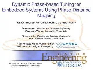
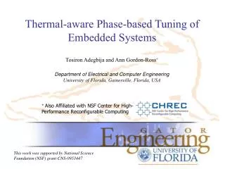
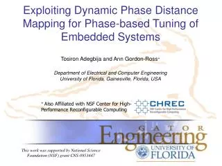
Exploiting Dynamic Phase Distance Mapping for Phase-based Tuning of Embedded Systems Tosiron Adegbija and Ann Gordon-Ross+ Department of Electrical and Computer Engineering University of Florida, Gainesville, Florida, USA + Also Affiliated with NSF Center for High-Performance Reconfigurable Computing This work was supported by National Science Foundation (NSF) grant CNS-0953447
Introduction and Motivation • Embedded systems are pervasive and have stringent design constraints • Constraints: Energy, size, real time, cost, etc. • System optimization is challenging due to numerous tunable parameters • Tunable parameters: parameters that can be changed • E.g., cache size, associativity, line size, clock frequency, etc. • Many combinations large design space • Multicore systems result in exponential increase in design space • Tradeoff design constraints • Design constraints (e.g., energy/performance) • Many Pareto optimal designs Energy What is the best design? Pareto optimal designs Execution time
Parameter Tuning • Parameter tuning determines appropriate parameter values • Appropriate parameter values meet optimization goals and satisfy design constraints • Different applications have different parameter value requirements • Parameter values must match the application’s requirements • Wastes up to 62% average energy (Gordon-Ross ‘05) if inappropriate • Parameter tuning specializes tunable parameters to the changing application requirements to meet optimization goals (e.g., lowest energy, best performance) • Configuration: specific combination of parameter values • Best configuration: configuration that most closely meets optimization goals • Parameter tuning is challenging • Large design space • Tuning overhead: energy/time consumed during tuning • Our contribution • Simplify parameter tuning, reduce tuning overhead
2KB 2KB 2KB 2KB Way shutdown Way concatenation 2KB 2KB 2KB 2KB Configurable Line size 2KB 2KB 2KB 2KB 8 KB, 2-way 4 KB, 2-way 2KB 2KB 2KB 2KB 8 KB, 4-way base cache 2KB 2KB 2KB 2KB 16 byte physical line size 8 KB, direct-mapped 2 KB, direct-mapped Parameter Tuning – Cache Tuning • Caches account for up to 50% of embedded system’s power. • Caches are a good candidate for energy optimization • Requires configurable cache A Highly Configurable Cache (Zhang ‘03) Tunable Asociativity Tunable Line Size Tunable Size
Executing in base configuration Download application Energy Cache Tuning Tunable cache TC Tuning hardware TC TC TC TC TC TC TC TC TC TC Dynamic Tuning • Dynamic tuning changes system parameter values at runtime • Dynamically determines best configuration with respect to optimization goals (e.g., lowest energy/best performance) • Requires tunable hardware and tuning hardware (tuner) • Tuner evaluates different configurations to determine the best configuration Cache energy savings of 62% on average! (Gordon-Ross ‘05) Lowest energy Execution time Microprocessor
Download application Tunable cache TC Tuning hardware TC TC TC TC TC TC TC TC TC TC Dynamic Tuning • Advantages • Adapts to the runtime operating environment and input stimuli • Specializes configurations to executing applications • Disadvantages • Large design space • Challenging to determine the best configuration • Runtime tuning overhead (e.g., energy, power, performance) • Energy consumed and additional execution time incurred during tuning Microprocessor
Base energy Energy Consumption Application-tuned Phase-tuned Change configuration Time Phase-based Tuning • Applications have dynamic requirements during execution • Different phases of execution • Tune when the phase changes, rather than when the application changes • Phase = a length of execution where application characteristics are relatively stable • Characteristics: cache misses, branch mispredictions, etc Time varying behavior for IPC, level one data cache hits, branch predictor hits, and power consumption for SPEC2000 gcc (using the integrate input set) Greater savings when tuning is phase-based, rather than application-based
Phase-based Tuning Variable length intervals Fixed length intervals Application x • Phase classification Profiler Conf1 Conf2 Conf4 Conf5 Conf3 How do we determine the best configuration for the different phases?
Energy Energy Execution time Execution time Previous Tuning Methods Exhaustive method Analytical method Heuristic method A lot of tuning overhead Energy Energy Energy Energy Execution time Possible Cache Configurations Possible Cache Configurations Possible Cache Configurations Less tuning overhead No tuning overhead but computationally complex/not dynamic Previous work proposed Phase Distance Mapping (PDM): a low-overhead and dynamic analytical method.
Phase Distance Mapping (PDM) Phase distance ranges Configuration change from Cb New phase Previously characterized phase Base phase Phase Pi Ci ?? d (Pb, Pi) Phase distance Distance windows Configuration distance
Phase Distance Mapping (PDM) Statically defined • PDM’s limitations Unknown applications/ general purpose systems? Needed to know/analyze applications a priori Distance windows Design time overhead!!! Base phase Most prominent application domain
Phase Tuning Architecture • Phase tuning architecture consists of phase characterization hardware • Phase characterization determines phase’s best configuration • Phase characterization hardware orchestrates PDM Processor core 1 Instruction cache Instruction cache L1 L1 Changes the tunable hardware and evaluates each configuration Data cache Data cache On-chip components Phase characterization hardware Tuner Main Memory Phase classification module Phase history table PDM module Distance window table Groups similar intervals into phases Processor core 2 Stores phase characteristics and configurations Determines a new phase’s best configuration
Contributions • We present DynaPDM: dynamic phase distance mapping • Alleviates design time effort • Shorter time-to-market • Maximizes energy delay product (EDP) savings • Defines distance windows during runtime • Dynamically designates base phase and calculates configuration distances • Specializes distance windows to dynamic system and application behavior • Low overhead, dynamic method for determining phase’s best configuration • DynaPDM evaluation • DynaPDM effectively determines best configuration with minimal designer effort • Applicable to general purpose embedded systems with disparate unknown applications (e.g., smartphones, tablets, etc.) • DynaPDM compared to PDM • Quantify DynaPDM’s EDP improvement over PDM • Achieves higher EDP savings than PDM without extensive a priori application analysis
Phase Characterization Used for comparison. Best configuration determined a priori or at runtime. • DynaPDM is part of phase characterization • Determines a phase, Pi’s best configuration Base phase, Pb Pb Phase classification Phases/ phase characteristics Phase history table CP1? Phase P1 executed Pb P1 CPb CPb x x CP1 P2 P1 P1 New phase, P1 x P3 P2 P4 P3 x x P4 DynaPDM CP1 P1 configuration, CP1
DynaPDM New phase, P1 d (Pb, P1) Distance window table ExecuteP1 in ConfigP1 CD3 DW3 Phase history table Calculate ConfigPi P1 ConfigP1 Create new DW Initialize DW
DynaPDM • Creating new distance windows • Windows defined by upper bound WinU and lower bound WinL • Phase distance D maps to a distance window if: WinL < D < WinU • Distance window size Sd = WinU – WinL • Empirically determined Sd = 0.5 as generally suitable for embedded processor applications • If D <Sd, WinL = 0, and WinU = Sd • WinUmax determines maximum number of new distance windows • If D > WinUmax, D maps to WinUmax < D < ∞ • Maximum number of distance windows = WinUmax/Sd • If Sd < D < WinUmax, • WinL = x | x ≤ D, x mod Sd = 0, x + Sd > D
DynaPDM • Initializing distance windows (DW) New DW? Set most recently used configuration as first phase’s initial configuration Tune cache size Tune cache parameters Tune associativity • n allows limited number of phase • executions to hone configurations closer • to the optimal • trades off improved configuration efficacy for • tuning overhead • depends on system’s application/phase • persistence Tune line size Execution j ≤ n? Power-of-two increments until EDP increases Yes No Defines DW’s configuration distance Stop tuning; Store lowest EDP configuration Continue tuning
Experimental Setup • Experiments modeled closely with PDM • Design space • Level 1 (L1) instruction and data caches: cache size (2kB 8kB); line size (16B64B); associativity (direct-mapped4-way) • Base cache configuration: • L1 instruction and data caches: cache size (8kB); line size (64B); associativity (4-way) • 16 workloads from EEMBC Multibench Suite • Image processing, MD5 checksum, networking, Huffman decoding • Each workload represented a phase • Simulations • GEM5 generated cache miss rates • McPAT calculated power consumption • Energy delay product (EDP) as evaluation metric = system_power * (total_phase_cycles/system_frequency)2
Experimental Setup • Workloads • Optimal configurations determined by exhaustive search • Used to compare DynaPDM and PDM results • Perl scripts implemented DynaPDM and PDM • Distribution of application phases used in experimental setup
Results DynaPDM’s configurations 1% of the optimal! 47% 28% • Used rotate-16x4Ms32w8 as base phase • EDP savings calculated with respect to base configuration • DynaPDM achieved 28% average EDP savings overall • Savings as high as 47% for 64M-rotatew2 • On average, within 1% of optimal • EDP improved over PDM by 8% Base phase DynaPDM improved over PDM and eliminated design-time effort!
Results • Effects of n = 3 on EDP normalized to optimal cache configurations • n = maximum number of phase executions Number of phase executions Determined optimal configurations in ≤ 3 executions! DynaPDM determined optimal configurations
Results Number of distance windows/ tuned phases/ tuning overhead • Tradeoffs of Sd with percentage of phases tuned at runtime Larger Sd Number of distance windows/ tuned phases/ tuning overhead Smaller Sd • Tradeoffs of Sd with percentage EDP savings Balance between tuning overhead and EDP savings Sd= 0.5 Larger Sd EDP savings
Conclusions • DynaPDM: Dynamic Phase Distance Mapping • Correlates known phase’s characteristics and best configuration with a new phase’s characteristics to determine new phase’s best configuration • Reduces tuning overhead • Compared DynaPDM with most relevant prior work: PDM • PDM required a priori knowledge of applications and extensive design-time effort • Not suitable for large or general purpose systems • DynaPDM eliminated design-time effort • DynaPDM achieved EDP savings of 28% and determined configurations within 1% of the optimal: 8% improvement over PDM • Future work • Evaluate DynaPDM’s scalability to many-core systems • Explore more complex systems with additional tunable parameters