Alluvial vs. bedrock channels
200 likes | 860 Vues
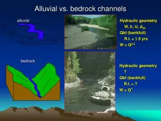
Alluvial vs. bedrock channels. Hydraulic geometry W, h, U, d 50 Qbf (bankfull) R.I. = 1.5 yrs W = Q 0.5. alluvial. bedrock. Hydraulic geometry ? Qbf (bankfull) R.I. = ? W = Q ?. Climate, straths, valley widths, and incision.

Alluvial vs. bedrock channels
E N D
Presentation Transcript
Alluvial vs. bedrock channels Hydraulic geometry W, h, U, d50Qbf (bankfull) R.I. = 1.5 yrsW = Q0.5 alluvial bedrock Hydraulic geometry ?Qbf (bankfull) R.I. = ?W = Q?
Climate, straths, valley widths, and incision (b) Bedload tools(Slingerland et al., 1997; Sklar and Dietrich, 1998) (a) Rock-type and wetting-drying cycles(Stock et al., 1996) (c) Climate Meyer et al., 1995 1. Stable Q, increased qs, cool climate 2. Flashy Q, decrease qsdry climate
Long profiles Q, W, d50
(1) Modeling bedrockincision 1 <a< 5/2 (2) Cf = dimensionless friction factor (3) c ~ 1 for small, steep drainages; Next slide (4) b ~ 0.5; Second slidecombine with conservation of massand steady, uniform flow Q=WhU (5) m/n = c(1-b) Calibration : Stock and Montgomery, 1999 Snyder et al., 2000 Much has been said about this equation and we have not heard the final word. It hasbeen an honest, exploratory attempt to reduce the complexities of a system we do notfully understand into a useful, simple expression that describes incision. Many of the earlier calibration studies assumed uniform incision (uplift) and an equilibrium(graded) profile…..we are motivated to calibrate and extract useful tectonic informationwhere incision (uplift) is not uniform along the profile.
Discharge – Area relationships Clearwater River c ~ 1 for wet climates, maybe best for bankfull c ~ 0.5 for arid climates
(Bedrock) channel widths valley widths Wbf Mitchell Wlf b for mixed bedrock-alluvial channels in N. NM ~ 0.5 (bankfull width) wrt drainage area ~ 0.6 (bankfull width) wrt discharge Tomkin et al., in press (Clearwater R.) b ~ 0.42 Snyder et al., 2000 b ~0.6-0.7
The equilibrium (steady-state) profile Rate of change of channel bed elevation= rate of uplift – incision rate (6) (7) When dz/dt = 0, Se = equilibrium slope ks is the profile steepness~ stream gradient index of Hack (1973) qis the profile concavity ~ 0.3 – 0.6 (Hack, 1957) (8) …. Tested in the field by the rate of incision reconstructed from terraces
Mean annualprecipitation Precipitationintensity Mean annualdischarge Peak annualprecipitation
Lab 4 Use EZ Profiler to extract a long profile Use EZ profiler to extract the flow accumulation values from the flow accumulationraster. Use the same polyline shape file that you used to extract the longprofile. Note what your raster cell size is – you need to know this to computethe drainage area. Bring the long profile (X vs. Z) and flow accumulation profile (X vs. A) into Excelor preferably SigmaPlot to calculate correct areas in km2 based on the cell size smooth the long profile (use the Lowess filter in SigmaPlot) throw out the area data that are very small numbers – these were not clipped from the channel correctly calculate channel gradient Deliverables (1) your spreadsheet or SigmaPlot worksheet (2) a plot with the long profile, SL index, and slope-area inset