Statistical tree estimation
Statistical tree estimation. Tandy Warnow. Topics: March 6-15. Stochastic models of sequence evolution Distance-based estimation Maximum parsimony tree estimation Maximum likelihood tree estimation Bayesian tree estimation. March 6, 2017. Two sequence evolution models:

Statistical tree estimation
E N D
Presentation Transcript
Statistical tree estimation Tandy Warnow
Topics: March 6-15 • Stochastic models of sequence evolution • Distance-based estimation • Maximum parsimony tree estimation • Maximum likelihood tree estimation • Bayesian tree estimation
March 6, 2017 • Two sequence evolution models: • Jukes-Cantor (for DNA) • Cavender-Farris-Neyman (for binary sequences) • Distance-based tree estimation • The Four Point Method • Naïve Quartet Method
-3 mil yrs AAGACTT AAGACTT -2 mil yrs AAGGCCT AAGGCCT AAGGCCT AAGGCCT TGGACTT TGGACTT TGGACTT TGGACTT -1 mil yrs AGGGCAT AGGGCAT AGGGCAT TAGCCCT TAGCCCT TAGCCCT AGCACTT AGCACTT AGCACTT today AGGGCAT TAGCCCA TAGACTT AGCACAA AGCGCTT AGGGCAT TAGCCCA TAGACTT AGCACAA AGCGCTT DNA Sequence Evolution
Phylogeny Problem U V W X Y AGGGCAT TAGCCCA TAGACTT TGCACAA TGCGCTT X U Y V W
Estimation of evolutionary trees as a statistical inverse problem • We can consider characters as properties that evolve down trees. • We observe the character states at the leaves, but the internal nodes of the tree also have states. • The challenge is to estimate the tree from the properties of the taxa at the leaves. This is enabled by characterizing the evolutionary process as accurately as we can.
Markov Model of Site Evolution Simplest (Jukes-Cantor, 1969): • The model tree T is binary and has substitution probabilities p(e) on each edge e. • The state at the root is randomly drawn from {A,C,T,G} (nucleotides) • If a site (position) changes on an edge, it changes with equal probability to each of the remaining states. • The evolutionary process is Markovian. More complex models (such as the General Time Reversible model, or the General Markov model) are also considered, often with little change to the theory.
Standard DNA site evolution models Figure 3.9 from Huson et al., 2010
Questions about model trees • Is the model tree topology identifiable? – yes • Are the branch lengths and other numeric parameters of the model tree identifiable? – yes • Is the root of the model tree identifiable? – no
Answers about model trees • Is the model tree topology identifiable? – yes • Are the branch lengths and other numeric parameters of the model tree identifiable? – yes • Is the root of the model tree identifiable? – no
Phylogeny estimation methods • Distance-based methods • Maximum parsimony • Maximum likelihood • Bayesian MCMC And other types that are not as commonly used
UPGMA • While |S|>2: • find pair x,y of closest taxa; • delete x • Recurse on S-{x} • Insert y as sibling to x • Return tree b c a d e
Performance criteria • Running time • Space • Statistical performance issues (e.g., statistical consistency and sequence length requirements) • “Topological accuracy” with respect to the underlying true tree, typically studied in simulation. • Accuracy with respect to a mathematical score (e.g. tree length or likelihood score) on real data
FN FN: false negative (missing edge) FP: false positive (incorrect edge) FP 50% error rate
Statistical Consistency error Data
Statistical models • Simple example: coin tosses. • Suppose your coin has probability p of turning up heads, and you want to estimate p. How do you do this?
Estimating p • Toss coin repeatedly • Let your estimateq be the fraction of the time you get a head • Obvious observation: q will approach p as the number of coin tosses increases • This algorithm is a statistically consistentestimator of p. That is, your error |q-p| goes to 0 (with high probability) as the number of coin tosses increases.
Another estimation problem • Suppose your coin is biased either towards heads or tails (so that p is not 1/2). • How do you determine which type of coin you have? • Same algorithm, but say “heads” if q>1/2, and “tails” if q<1/2. For large enough number of coin tosses, your answer will be correct with high probability.
Markov models of character evolution down trees • The character might be binary, indicating absence or presence of some property at each node in the tree. • The character might be multi-state, taking on one of a specific set of possible states. Typical examples in biology: the nucleotide in a particular position within a multiple sequence alignment. • A probabilistic model of character evolution describes a random process by which a character changes state on each edge of the tree. Thus it consists of a tree T and associated parameters that determine these probabilities. • The “Markov” property assumes that the state a character attains at a node v is determined only by the state at the immediate ancestor of v, and not also by states before then.
Binary characters • Simplest type of character: presence (1) or absence (0). • How do we model the presence or absence of a property?
Cavender-Farris-Neyman (CFN) • Models binary sequence evolution • For each edge e, there is a probability p(e) of the property “changing state” (going from 0 to 1, or vice-versa), with 0<p(e)<0.5 (to ensure that unrooted CFN tree topologies are identifiable). • Every position evolves under the same process, independently of the others.
Estimating trees under statistical models… • Instead of directly estimating the tree, we try to estimate the process itself. • For example, we try to estimate the probability that two leaves will have different states for a random character.
CFN pattern probabilities • Let x and y denote nodes in the tree, and pxy denote the probability that x and y exhibit different states. • Theorem: Let pi be the substitution probability for edge ei, and let x and y be connected by path e1e2e3…ek. Then 1-2pxy = (1-2p1)(1-2p2)…(1-2pk)
And then take logarithms • The theorem gave us: 1-2pxy = (1-2p1)(1-2p2)…(1-2pk) • If we take logarithms, we obtain ln(1-2pxy)= ln(1-2p1) + ln(1-2p2)+…+ln(1-2pk) • Since these probabilities lie between 0 and 0.5, these logarithms are all negative. So let’s multiply by -1 to get positive numbers.
An additive matrix! • Consider a matrix D(x,y) = -ln(1-2pxy) • This matrix is additive (i.e., fits a tree exactly)! • Can we estimate this additive matrix from what we observe at the leaves of the tree? • Key issue: how to estimate pxy. • (Recall how to estimate the probability of a head…)
Estimating CFN distances • Consider dij= -1/2 ln(1-2H(i,j)/k), where k is the number of characters, and H(i,j) is the Hamming distance between sequences si and sj. • Theorem: as k increases, dij converges to Dij = -1/2 ln(1-2pij), which is an additive matrix.
CFN tree estimation • Step 1: Compute Hamming distances • Step 2: Correct the Hamming distances, using the CFN distance calculation • Step 3: Use distance-based method (neighbor joining, naïve quartet method, etc.)
Four Point Method • Task: Given 4x4 dissimilarity matrix, compute a tree on four leaves • Solution: Compute the three pairwise sums, and take the split ij|kl that gives the minimum! • When is this guaranteed accurate?
Error tolerance for FPM • Suppose every pairwise distance is estimated well enough (within f/2, for f the minimum length of any edge). • Then the Four Point Method returns the correct tree (i.e., ij+kl remains the minimum)
Naïve Quartet Method • Compute the tree on each quartet using the four-point condition • Merge them into a tree on the entire set if they are compatible: • Find a sibling pair A,B • Recurse on S-{A} • If S-{A} has a tree T, insert A into T by making A a sibling to B, and return the tree
Error tolerance for NQM • Suppose every pairwise distance is estimated well enough (within f/2, for f the minimum length of any edge). • Then the Four Point Method returns the correct tree on every quartet. • And so all quartet trees are compatible, and NQM returns the true tree.
In other words: • The NQM method is statistically consistent methods for estimating CFN trees! • Plus it is polynomial time! Can we use it on DNA sequences?
Standard DNA site evolution models Figure 3.9 from Huson et al., 2010
Jukes-Cantor DNA model • Character states are A,C,T,G (nucleotides). • All substitutions have equal probability. • On each edge e, there is a value p(e) indicating the probability of change from one nucleotide to another on the edge, with 0<p(e)<0.75 (to ensure that JC trees are identifiable). • The state (nucleotide) at the root is random (all nucleotides occur with equal probability). • All the positions in the sequence evolve identically and independently.
Jukes-Cantor distances • Dij = -3/4 ln(1-4/3 H(i,j)/k)) where k is the sequence length • These distances converge to an additive matrix, just as with CFN distances
UPGMA • While |S|>2: • find pair x,y of closest taxa; • delete x • Recurse on S-{x} • Insert y as sibling to x • Return tree b c a d e
UPGMA Works when evolution is “clocklike” b c a d e
UPGMA Fails to produce true tree if evolution deviates too much from a clock! b c a d e
Statistical Consistency error Data
UPGMA is NOT statistically consistent! error Data
Better distance-based methods (all statistically consistent under JC) • Neighbor Joining • Minimum Evolution • Weighted Neighbor Joining • Bio-NJ • DCM-NJ • And others
Quantifying Error FN FN: false negative (missing edge) FP: false positive (incorrect edge) 50% error rate FP
Neighbor joining has poor performance on large diameter trees [Nakhleh et al. ISMB 2001] Simulation study based upon fixed edge lengths, K2P model of evolution, sequence lengths fixed to 1000 nucleotides. Error rates reflect proportion of incorrect edges in inferred trees. 0.8 NJ 0.6 Error Rate 0.4 0.2 0 0 400 800 1200 1600 No. Taxa
Summary so far • Distance-based methods are generally polynomial time, and can be statistically consistent under standard sequence evolution models. • Yet they can have high error under high rates of sequence evolution. What are the options?
Homework due tomorrow • Be able to calculate CFN distances from sequence data • Be able to apply the Four Point Method to construct a tree from a set of 4 binary sequences