Projecting Quality
180 likes | 284 Vues
Learn about projecting field problems with static & dynamic models, Weibull distribution, and Rayleigh Curve in software quality assurance. Understand how to estimate remaining issues in a product life cycle using advanced mathematical approaches.

Projecting Quality
E N D
Presentation Transcript
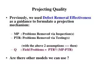
Projecting Quality • Previously, we used Defect Removal Effectiveness as a guidance to formulate a projection mechanism: • MP : Problems Removed via Inspection(s) • PTR: Problems Removed via Testing(s) (with the above 2 assumptions ---- then) • Q : Field Problems = PTR2/ (MP-PTR) • Are there other models we can use ?
Projecting Field Problems • 2 Basic Models : • Static Model : • # of Field Problem or Q = f ( x1, x2, - - - - -, xn) where x’s are a set of parameters such as size of the software, skills of the people, development schedule, etc. • The coefficients of x’s used in the computation come from previous, similar projects. • The computation of # of Field Problems for the project is assumed to be one from a population of similar projects.
Projecting Field Problems • Dynamic Model : • Estimate is based on multiple measurements taken from the project of interest, not from other projects, but from the current project • It is more specific to the project or product. • It is often expressed in terms of time. • We will use one such model to simulate the complete product life cycle.
Weibull Distribution family • Has been used by other disciplines for reliability analysis and projecting the defect as a function of time. • The probability density function : f(t) = (m/t) * ((t/c)**m) * (e ** -((t/c)**m) ) = (m/t) (t/c)m e (–t/c) **m • m is a parameter that shapes the curve • t is the time • c is a parameter which is a function of t when the curve reaches maximum point. • The cumulative distribution function : (integrate the above) F(t) = 1 – (e** -((t/c)**m) )
Weibull Curves (with differing m’s) f(t) = (m/t) * ((t/c)**m) * ( e** (-(t/c)**m) ) m= 8 problems found m= 2 m= 4 m= 1 t: some unit of time
Rayleigh Curve • A special case of Weibull curve where m=2 is called the Rayleigh curve f(t) = (2/t) * ((t/c)**2) * ( e** (-(t/c)**2) ) At tmax , the area under the curve is ~39.3% problems found m= 2 tmax t: some unit of time
Rayleigh Curve • The area under the f(t) curve (normalized to a total of 1) is the (% of)accumulative total problems found through some time. The integral of f(t) is the cumulative distribution function: F(t) = 1 - (e** (-(t/c)**2) ) total problems found t : time units
Applying Rayleigh Curve concept to Discrete Measurements • Let’s map software defect removal activities into the Rayleigh Curve: (Some projects have found the mapping to hold) Io = requirement inspection I1 = design inspection I2 = code inspection UT= unit testing CT = component testing ST = system testing FP = field problems problems found I I CT ST FP or Q I UT 0 1 2 t : product life phases
Projection of Field Problems with Rayleigh Curve • If your project appears to show a Rayleigh curve through the first couple of inspections • Continue to track against the curve • See if the peak point is close to UT phase. Assign that phase or time as the point where f(t) reaches the max point. • Use that max time to compute the value of “c”for the Rayleigh curve for your product: c= t * 2 (see next chart) • f(t) = (2/t) * ((t/c)**2) * (e** (-(t/c)**2)) max
Solving for the “c” parameter • A Way to solve for the parameter, c, in Rayleigh curve • Take the first derivative of f(t) and set it to 0 to find the time at which f(t) peaks. • d[f(t)] = d[(2/t) * ((t/c)**2) * (e**(-(t/c)**2)) ] • = d[ (2t/(c**2)) * (e**(-(t/c)**2)) ] • = (2t/(c**2) ) d[e**(-(t/c)**2)] + d[2t/(c**2)](e**(-(t/c)**2)) • = (2t/(c**2)) [(e**(-(t/c)**2)) d[-(t/c)**2] + {second part} • = (2t/(c**2))[(e**(-(t/c)**2)) * (-2t/c**2)] + {second part} • = ((-4t**2)/(c**4)) (e**(-(t/c)**2)) + {second part} • = {first part} + (2/(c**2)) (e**(-(t/c)**2) • = (e**(-(t/c)**2)) *[( (-4t**2)/c**4)) + (2/c**2)] = 0 • (-4t**2)/(c**4) +(2/c**2) = 0 • (-4t**2)/(c**4) = - (2/c**2) • -(2t**2) = - (c**2) • t**2 = (c**2)/2 • t = c / (sqrt(2)) look for ‘max’
Try an Example with Rayleigh Curve • Assume the following information (collected data) • I0 : at time 1 with 9 problems found • I1 : at time 2 with 12 problems found • I2 : at time 3 with 17 problems found • UT : at time 4 with 10 problems found • CT : at time 5 with 6 problems found • ST : at time 6 with 3 problems found • FP : problems in remaining time (field problems) • tmax is approximated at time unit 3, or I2, in this case = total of 57 problems
Example Continued • Using the previous equation : tmax = c /sqrt(2) • c = tmax * sqrt(2) = 3 * 1.41 = 4.23 • Use the accumulative F(t)= 1 – e**(-(t/c)**2) • F(6) = 1 – e**(-(6/4.23)**2) = 1 – e**(-1.99) = 1- (.135) = .865 • Since 1 is the total area under the curve, the remaining area under the curve is .135. • Also since .865 is approximately equal to the total problems found up to end of system test, which is 57 problems, then the total life cycle is estimated at 66 problems. (57/.865 = 66) • Thus the remaining problems in the field is estimated at 66-57 = 9 problems. • FP (field problems) is estimated at 9 problems
Compare with the Previous Estimation Method • Consider the previous estimation of Field Problems Q = PTR/(μ-1) = PTR / [(MP/PTR) -1] = PTR2/(MP-PTR) • Substituting the numbers : • Q = 192/(38 -19) • Q = 361/19 = 19 problems • Note the difference between the 2 estimates with the same assumed problems found rates : • Q with Rayleigh Curve approach estimated at 9 problems • Q with the PTR2/(MP-PTR) estimated at 19 problems. (Remember the “earlier” estimate assumed MP/TD = PTR/(TD-MP) which in this case 38/66 does NOT equal 19/28)
Estimates • Remember that these are still estimates and not all the conditions are known, yet. • Two assumptions are used in using the Rayleigh curve to model quality of software: • The defect rate observed during development activities is highly correlated to the defect rate in the field. • Given the same error injection rate, then the more defects discovered early in the development cycle, the fewer will remain in the system at later stages.
Correlating Development Phase I0-inspection, Defect Rate with Field Defect rate Rank field defect rate by module Rank I0 by module (Diff)2 Diff -3 -18 -22 -5 . . . +13 9 324 484 25 . . . 169 4 20 25 9 . . . 52 1 2 3 4 . . . 65 Spearman’s Rank Order Correlation coefficient = 1 – {[6* Σ(diff)2] / [n *(n2-1)]} Using this technique, book author found low correlation for I0, I1 to field defects and higher correlation of I2, CT, and ST to field defects
More “thoughts” illustrated with Rayleigh curve Using the same process of error removals for a set of modules, we have been noticing that if we find lots of bugs in a module, X, relative to other modules, then that same module, X, tends to be more error prone (have high # of bugs) in the field also. [ A uniform upward shift effect - no shape change] # of Defects found More error prone module A “typical” module product release day Time
More “thoughts” illustrated with Rayleigh Curve We have also justified the concept of finding more bugs prior to release is a good scenario because less will be in the product after release. So if more bugs are found in a module, X, relative to other modules prior to release should be a good sign. How does that relate to the comments on a module with lots of bugs found prior to release tends to be the same module that is error prone in the field? [ A change in shape of the curve ---due to modified process ] Modified or improved process and the number of problems removed shifted to the front, resulting in less problems detected after release. Original process and the number of problem found Product release
Reliability and Predictive Validity of Models • Reliability of the Model refers to the confidence we have of the model in terms of its estimates. • Dos the output from the model vary greatly from one input set to another input set? • Predictive Validity of the Model refers to the accuracy of the model estimates, especially compared to empirical data • The author found that using Rayleigh curve model across different systems such as AS/400, S/38/ and S/36 data showed that the field problems discovery rate is consistently underestimated. The model had to be adjusted to set m= 1.8 for the IBM mid-range systems.