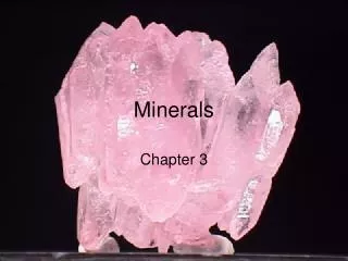
Chapter 3 Crystalline Structure–Perfection

1. Chapter3Crystalline Structure–Perfection

2. 3.1 SevenSystems and Fourteen Lattices Consider the atomic-scale structure of the engineering materials of which they are crystalline; that is, the atoms of the materials are arranged in a regular and repeating manner. Figure 3.1Various structural units that describe the schematic crystalline structure. The simplest structural unit is the unit cell. Fundamental crystal geometry has the seven crystal systems and 14 crystal lattices. The crystalline structures of most metals belong to one of three relatively simple types. Ceramics which have variety of chemical compositions, exhibit variety of crystalline structures. The basic Glass is noncrystalline, and polymers may have as much as 50 to 100% of their volume noncrystalline. There may be several different shapes of the combination of the circles, however, there is only one which is the basic.

3. Nomenclatures : Z Lattice constants or lattice parameters; α, b and c are the unit length along X, Y and Z axes, respectively.. α,β, and γare the angles between the crystallographic axes.. Figure 3.2 Geometry of a general unit cell. Unit cell Y These six parameters are called lattice constants or lattice parameters. X The lattice parameters a, b, and c are unit cell edge lengths. The lattice parameters α, β, and γ are angles between adjacent unit-cell axes, where α is the angle viewed along the a axis (i.e., the angle between the b and c axes). The inequality sign(≠) means that equality is not required.

4. Seven Crystal Systems and 14 Bravais’ Lattices All possible structures reduce to a small number of basic unit-cell geometries, which is demonstrated in two ways. First, there are only seven unique unit-cell shape that can be stacked together to fill three-dimensional space. These are called Seven Crystal Systems. Second, consider the points where the atoms are stacked in a given unit-cell. These points are called lattice points. And there is 14 possible ways of arrangement of the points, called 14 Bravais’ Lattices.

5. The lattice parameters a, b, and c are unit cell edge lengths. The lattice parameters α, β, and γ are angles between adjacent unit-cell axes, where α is the angle viewed along the a axis (i.e., the angle between the b and c axes). The inequality sign(≠) means that equality is not required.

6. Lattice points in simple cubic Figure 3.3 The simple cubic lattice becomes the simple cubic crystal structure when an atom is placed on each lattice point. Simple cubic crystal with atoms on each lattice point Every crystal can be drawn in these two different ways, however, “lattice point” is more convenient for practical use.

7. (14 possible way of arrangement of the lattice points in unit-cells.)

8. Examples and Practice Problems : Students are asked to review the “Example” of 3.1 and solve the “Practice Problem” of 3.1 in the text.

9. 3.2 Metal Structures Mostmetals have 3 structures; BCC, FCC and HCP. Figure 3.4Body-centered cubic (bcc) structure for metals showing (a) the arrangement of lattice points for a unit cell, (b) the actual packing of atoms (represented as hard spheres) within the unit cell, and (c) the repeating bcc structure, equivalent to many adjacent unit cells. BCC crystal structure Atomic Packing Factor : 0.68% Atoms/unit cell : 2 Most Compact Atomic Plane : {110} Most Closest Atomic Direction : 〈111〉 These above parameters are very useful to understand thermal, physical and mechanical properties of the metals. (discussed more later)

10. Interstitial voids in cubic crystals In FCC, there are two different interstitial voids; 1). Octahedral void : r = 0.414 R 2). Tetrahedral void : r = 0.225 R In BCC, there are two different interstitial voids; 1). Octahedral void : r = 0.154 R 2). Tetrahedral void : r = 0.291 R Students are asked to calculate the size of the four voids. r = radius of the interstitial atom. R= radius of the matrix atom.

11. FCC crystal structure Atomic Packing Factor : 0.74% Atoms/unit cell : 4 Most Compact Atomic Plane : {111} Most Closest Atomic Direction : 〈110〉 Figure 3.5 Face-centered cubic (fcc) structure for metals showing (a) the arrangement of lattice points for a unit cell, (b) the actual packing of atoms within the unit cell, and (c) the repeating fcc structure, equivalent to many adjacent unit cells.

12. Explain the physical meaning of the calculated values !

13. (This atom is locating at the center of the cell.) Figure 3.6Hexagonal close-packed (hcp) structure for metals showing (a) the arrangement of atom centers relative to lattice points for a unit cell. There are two atoms per lattice point (note the outlined example). (b) The actual packing of atoms within the unit cell. Note that the atom in the midplane extends beyond the unit-cell boundaries. (c) The repeating hcp structure, equivalent to many adjacent unit cells. [Part (c) courtesy of Accelrys, Inc.] HCP crystal structure Atomic Packing Factor : 0.74% Atoms/unit cell : 2 Most Compact Atomic Plane : (0001) Most Closest Atomic Direction : 〈0110〉

14. The relationship between edge length(a) and atomic radius(r) can be easily calculated by understanding the configuration of the crystals. That is, one has to know the atomic positions and the relative location of the atoms in the unit-cell of each crystal.

15. FCC PF=0.74 HCP PF=0.74 Atomic stacking sequence : ABABAB on (0001) planes Figure 3.7Comparison of the fcc and hcp structures. They are each efficient stackings of close-packed planes. The difference between the two structures is the different stacking sequences. Atom stacking sequence : ABCABC on {111} planes (111) Explain the difference in the mechanical behaviors using slip system concept. (0001)

16. Examples and Practice Problems : Students are asked to review the “Example” of 3.2 and solve the “Practice Problem” of 3.2 and3.3 in the text.

17. 3.3 Ceramic Structures In ceramic, there is Ionic Packing Factor (IPF), similar to atomic packing factor in metals, Variety of chemical composition Figure 3.8 Cesium chloride (CsCl) unit cell showing (a) ion positions and the two ions per lattice point and (b) full-size ions. Note that the Cs+−Cl− pair associated with a given lattice point is not a molecule because the ionic bonding is nondirectional and because a given Cs+is equally bonded to eight adjacent Cl−, and vice versa Many different crystal structures Explain some typical structures Consider CsCl, simplest chemical formular For one kind of ion, it is simple cubic, however, for ionic compound, it is BCC type and it is representing the CsCl type ionic crystals. One anion and one cation are involved for the formation of ceramic. This means two ions have same charge but opposite character.

18. NaCl structure This structure can be viewed as the intertwining of two fcc structures one of sodium ions and one of chlorine ions. Figure 3.9Sodium chloride (NaCl) structure showing (a) ion positions in a unit cell, (b) full-size ions, and (c) many adjacent unit cells. Many important ceramic materials have this type of structure; MgO, CaO, FeO, and NiO, ect. This is same as of the case CsCl, i.e., one anion and one cation are involved for the formation of ceramic. This means two ions have same charge but opposite character.

19. MX2 type ceramics ; CaF2 Two different ions have different charge values. There are 12ions (4 Ca2+ and 8 F-) perunitcell. Figure 3.10Fluorite (CaF2) unit cell showing (a) ion positions and (b) full-size ions. At the center of the unit cell, there is no ion, means that it is a void. This void plays an important role in nuclear-materials technology. UO2 is a reactor fuel that can accommodate fission products such as helium gas . This gas stays in the void to eliminate troublesome swelling.

20. 4- Another example of MX2 type ceramics : Si02 SiO4 tetrahedron SiO2 is widely available law materials in the earth’s crust. Silica represents large fraction of the ceramic materials. For this reason, the structure of SiO2 is important. However, the structure is not simple. Figure 3.11The cristobalite (SiO2) unit cell showing (a) ion positions, (b) full-size ions, and (c) the connectivity of tetrahedra. In the schematic, each tetrahedron has a Si4+at its center. In addition, an O2−would be at each corner of each tetrahedron and is shared with an adjacent tetrahedron. [Part (c) courtesy of Accelrys, Inc.] This figure shows the structure of cristobalite, one of the many different structures of SiO2, There are 24 ions(8 Si4+ and 16 O2-) per unit cell of fcc type. In spit of the large number of unit cell needed to describe this structure, it is perhaps the simplest of the various crystallographic form of SiO2.

21. As Fe has an allotropic transformation with temperature, silica also has the different crystal structures with temperature. But even though Si02 crystal structures are different, the same basic SiO4 tetrahedra is the connecting element of the crystals. Figure 3.12Many crystallographic forms of SiO2are stable as they are heated from room temperature to melting temperature. Each form represents a different way to connect adjacent tetrahedra. 4-

22. M2X3 type ceramics : Al2O3 Figure 3.13 The corundum (Al2O3) unit cell is shown superimposed on the repeated stacking of layers of close-packed O2−ions. The Al3+ions fill two-thirds of the small (octahedral) interstices between adjacent layers. Corundum (Al2O3) is an important example of M2X3 as shown in above figure. This structure is in a rhombohedral Bravais lattice, but it closely approximates a hexagonal lattice. There are 30 ions (12 Al3+ and 18 O2-) per unit cell.

23. Kaolinite [2(OH)4Al2Si2O5] is a hydrated aluminosilicate and a good example of a clay mineral. The structure is typical of sheet silicates. (See Fig. 3.15 in next slide.) This Kaolinite structure is made by the breaking up the continuity of the SiO4 with the additional oxides. Figure 3.14 Exploded view of the kaolinite unit cell, 2(OH)4Al2Si2O5. 4-

24. Figure 3.15 Transmission electron micrograph of the structure of clay platelets. This microscopic-scale structure is a clear view of the layered crystal structure shown in Figure 3.14.

25. Graphite is the stable room temperature crystal structure of carbon. Figure 3.16 (a) An exploded view of the graphite (C) unit cell (b) A schematic of the nature of graphite’s layered structure. Graphite is monatomic of carbon, but it is much more ceramiclike than metallic. Although, the hexagonal rings of carbon atoms are strongly bonded by covalent bonds, the bonds between layer, however, of the van der Waals type, to give friable nature and to be applicable as a useful “dry” lubricant. (Compare the structure and propertie between graphite and diamond.)

26. Figure 3.17(a) illustrates the structure of a C60 molecule. This unique structure of carbon was discovered during experiment on the laser vaporization of carbon in a carrier gas of helium. Since the structure is similar to that of geodesic dome constructed by Buckminister Fuller, American architect, it is called buckministerfullerene (simply fullerene) or buckyball (by its shape of soccer ball). This structure is a spherical molecule of polyhedron composed or 5-fold and 6-fold faces. Figure 3.17(a) C60molecule, or buckyball. (b) Cylindrical array of hexagonal rings of carbon atoms, or buckytube. Subsequent research has led to the synthesis of a wide variety of structures fdor a wide range of fullerenes. Buckyballs have been synthesized with the formula Cn, where n cantake large even numbers as 240 and 540. From extensive research it is realized that cylindrical curvature can be obtained, simply rolling the hexagonal graphite sheets, to form a buckytube. 12 pentagons, 20 hexagons form a buckyball These materials have unique chemical and physical properties. Buckytube (nanotube) has the theoretical promise of being the highest-strength reinforcing fibers available for the advanced composites.

27. Examples and Practice Problems : Students are asked to review the “Example” of 3.3, and3.4 and solve the “Practice Problem” of 3.4 and3.5 in the text.

28. H C 3.4 Polymeric Structure Figure 3.18 Arrangement of polymeric chains in the unit cell of polyethylene. The dark spheres are carbon atoms, and the light spheres are hydrogen atoms. The unit-cell dimensions are 0.255 nm × 0.494 nm × 0.741 nm. Polymer : chain-like structure of long polymeric molecules. ↓ Difficult to be crystalline structure ↓ Structural description is not easy, it is beyond the scope of this lecture orthorhombic unit cell This figure illustrates the shape of polyethylene (C2H4)n which is chemically simple. However, long chain molecules fold back and forth to become complicated shape. It may have an orthorhombic unit cell to show a crystal character over a large volume.

29. Single crystals of polyethylene are difficult to grow. If polyethylene is produced by cooling from a dilute solution, they tends to be thin plates, about 10 nm thick. Figure 3.19 Weaving-like pattern of folded polymeric chains that occurs in thin crystal platelets of polyethylene. Since polymer chains are generally several hundred nanometers long, the chain must be folded back and forth in as sort of atomic-scale weaving (crystal like) in this thin plate.

30. Examples and Practice Problems : Students are asked to review the “Example” of 3.5 and solve the “Practice Problem” of 3.6 in the text.

31. 3.5 Semiconductor structure The technological and cultural revolution created by the many scientific products based on the modern integrated circuit begins with single crystals of exceptionally high chemical purity and structural perfection. The vast majority of integrated circuits are produced on thin slices (wafer) of silicon single crystal. Nowadays 300mm dia. silicon rod is produced with 10μm/s growth rate by the so called “Czochralski technology”. Semiconductor industry induces the crystal grower to produce as large a diameter crystal as possible because of the economic view point. Even though theory implies perfect crystal, in practice, all structures are subject to various imperfections. (Defects will be discussed in Ch. 4) Single crystals of Si, Ge, and Sn are the elemental semiconductors (VI A group) and they have the structure of diamond cubic. (See Fig. 3.20 in next slide) A small number of elements adjacent group IV A forms compound semiconductors, which tend to be MX-type compounds with combinations of atoms having an average valence of 4+. For example, GaAs (III-V compound) combines Ga3+ with As5+ , and CdS (II-VI compound) combines Cd2+ and S6+ . Many of these MX compounds crystallize in a structure closely related to the diamond cubic. (This compound semiconductor is discussed in Chapter 13.)

33. As it has been explained in the previous slide, diamond cubic crystal is the most important crystal structure of the semi-conducting materials. Figure 3.20 Diamond cubic unit cell showing (a) atom positions. There are two atoms per lattice point (note the outlined example). Each atom is tetrahedrally coordinated. (b) The actual packing of full-size atoms associated with the unit cell. One kind of atom forms diamond structure. The atomic arrangements in the unit cell is quite similar to that of diamond which is crystallized with carbon. However, in this crystal, it is not carbon but Si, Ge and gray Sn. So it is called “diamond cubic”. : Elemental semiconductors

34. Figure 3.21Zinc blende (ZnS) unit cell showing (a) ion positions. There are two ions per lattice point (note the outlined example). Compare this structure with the diamond cubic structure (Figure 3.20a). (b) The actual packing of full-size ions associated with the unit cell. Two different kinds of ions form diamond structure, so it is called Zinc blende. : compound semiconductors

35. Examples and Practice Problems : Students are asked to review the “Example” of 3.6 and 3.7 and solve the “Practice Problem” of 3.7 and 3.8 in the text.

36. 3.6 Lattice Positions, Directions, and Planes Lattice position Introduce basic rules for describing geometry in and around a unit cell. Figure 3.22 Notation for lattice positions. Some important vocabularies : 1). Lattice positions: sameas the position in the angular co-ordinates, xyz. The detailed examples are shown in Figure 3.22.

37. Some important vocabularies : 2). Lattice translations: One aspect of the nature of crystalline structure is that a given lattice position in a given unit cell is structur-ally equivalent to the same position in any other unit cell of the same structure. A’’ Figure 3.23Lattice translations connect structurally equivalent positions (e.g., the body center) in various unit cells. This operation is called Lattice translation. A A’

38. Some important vocabularies : Figure 3.24Notation for lattice directions. Note that parallel [uvw] directions (e.g., [111]) share the same notation because only the origin is shifted. Directions are in the square brackets. 3. Lattice directions : Indications of the directions from one lattice position to the other in a given crystal structure. “Position” is not in any bracket. Theses directions are always expressed as sets of integers, which are obtained by identifying the smallest integer positionsintercepted by the line from the origin of the crystallographic axes and they are in the square brackets.

39. Some important vocabularies : Figure 3.25 Family of directions, (111), representing all body diagonals for adjacent unit cells in the cubic system. 4. Family directions : All the directions shown in the figure are for the diagonal directions, which are all equivalent. The angle between two different directions is ; D• D’ = D D’ cos δ The shape of the bracket for family direction.

40. Miller indices : Todescribe lattice directions and lattice planes, we need to have certain symbols. These are called Miller indices and are expressed as a set of integers. For general expression, h,k, and l are used for cubic. The angle between two different directions In further chapters, especially when dealing with calculation of mechanical properties, it will be useful to know the angle between directions. In general, the angles between directions can be determined by careful visualization and trigonometric calculation. In the frequently encountered cubic system, the angle can be determined from the relatively simple calculation of a dot product of two vectors. Taking directions [u v w] and [u’ v’ w’] as vectors D = ua + vb +wc and D’ = u’a + v’b +w’c, you can determine the angle, δ, between these two directions by D• D’ = D D’ cos δ uu’ + vv’ + ww’ or, cos δ= √u2+v2+w2 √(u’)2+(v’)2+(w’)2

41. Linear density of atoms along a given direction Linear density of atoms : number of atoms whose centers are passed along a given unit length of direction. For the understanding of the motion of dislocations, the linear density of atoms is very important factor. A reasonable approach in the case where atoms are uniformly spaced along a given direction is to determine the repeat distance, r, between adjacent two atoms (in other words, in the distance r, there two atomic radii or one atom). Therefore, the linear density is simply the inverse, r -1. One needs to convert this number (r -1), into # atoms/cm.

42. How to determine the plane notation using : intercept position in each axis 1). 2). Take the inverse of the intercepts; 2/1, 1/1, 1/∞ (210) Figure 3.26Notation for lattice planes. (a) The (210) plane illustrates Miller indices (hkl). (b) Additional examples. 3). take the least common multiple. (take the least common multiple) Miller Indices are used for the notation of the lattice planes.

43. For HCP crystal system, different from the cubic, since there are 4 axes, Miller indices are; h, k, i, l. Figure 3.27 Miller–Bravais indices (hkil) for the hexagonal system. α1 +α2 +α3 = 0 h + k = -i α1α2α3c : Same method as in cubic crystal

44. For each plane : (h k l) Figure 3.28 Family of planes, {100}, representing all faces of unit cells in the cubic system. For family of planes : {h k l}

45. Examples and Practice Problems : Students are asked to review the “Example” of 3.8 ~ 3.19 and solve the “Practice Problem” of 3.9 ~ 3.21 in the text.

46. 3.7 X-Ray Diffraction Even for the visible light, if the condition is met, all the scattered light can be diffracted as in the figure . However, this is not same as the x-ray diffraction. Figure 3.29Diffraction grating for visible light. Scratch lines in the glass plate serve as light-scattering centers. Scratches 1μm 1μm = (1/million)m = 103 nm 1 nm = (1/billion)m Visible light The wave length of visible light ~ 1μm. Therefore, the visible light can be diffracted by the 1μm scratches evenly distributed.

47. Figure 3.30Electromagnetic radiation spectrum. X-radiation represents that portion with wavelengths around 0.1 nm.

48. Incident beam angle Figure 3.31Geometry for diffraction of x-radiation. The crystal structure is a three-dimensional diffraction grating. Bragg’s law (nλ = 2d sin θ) describes the diffraction condition. 1). 2). 3). Bragg Equation or Bragg’s law : Basic condition for diffraction : λ and d are similar! (When the Bragg’s condition is satisfied, the incident beam angle is the diffraction angle)

49. Figure 3.32Relationship of the Bragg angle (θ) and the experimentally measured diffraction angle (2θ). Bragg’s law defines the diffraction condition for primitive unit cells; that is those Bravais lattices with lattice points only at unit-cell corners, such as simple cubic and simple tetragonal. Crystal structures with nonprimative unit cells have atoms at additional lattice sites located along a unit-cell edge, within a unit-cell face, or in the interior of the unit cell. The extra scattering centers can cause out-of-phase scattering to occur at certain Bragg angles. The result is that some of the diffraction predicted by Bragg Equation does not occur. An example of this effect is given in Table 3.4 (next slide), which gives the reflection rules for the common metal structures. These rules show which sets of Miller indices do not produce diffraction as predicted by Bragg’s law.

50. As it has been explained in the previous slide, Table 3.4 (next slide) shows the reflection rules for nonprimative unit cells or the common metal structures. These rules show which sets of Miller indices do not produce diffraction as predicted by Bragg’s law. Where a and c are the lattice parameters. α In cubic, the spacing between adjacent h k l planes is : dhkl = √h2 + k2 + l2 For more complex unit-cell shapes, the relationship is more complex. For a hexagonal system, Where α and c are the lattice parameters.