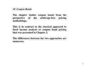
Time
Table 10.1: The Cash Flows to a Typical Coupon Bond with Price B (0), Principal L, Coupon C and Maturity T. 0 1 2 … T | | | | B (0) C C … C Coupons L Principal. Time. coupon rate c = 1+C/L. Table 10.2: An Example of a Time 0 Zero-Coupon Bond Price Curve. P(0,4) = .923845

Time
E N D
Presentation Transcript
Table 10.1: The Cash Flows to a Typical Coupon Bond with Price B(0), Principal L, Coupon C and Maturity T 0 1 2 … T | | | | B(0) C C … C Coupons L Principal Time coupon rate c = 1+C/L
Table 10.2: An Example of a Time 0 Zero-Coupon Bond Price Curve P(0,4) = .923845 P(0,3) = .942322 P(0,2) = .961169 P(0,1) = .980392
1.054597 .985301 1 1 1.037958 1/2 .967826 1.016031 .984222 1.054597 1 1/2 1/2 .981381 1.02 1 1 .947497 .965127 1.059125 1.017606 .982699 1 .982456 1 1.037958 1 1/2 1/2 1/2 .960529 1 1.020393 B(0) .980015 1.059125 1 P(0,4) .923845 1/2 .977778 P(0,3) 1 .942322 1 = r(0) = 1.02 P(0,2) .961169 P(0,1) .980392 1.062869 P(0,0) 1 .983134 1.042854 1/2 1 1 .962414 1/2 1.019193 .981169 1.02 1/2 1.062869 1 1/2 .937148 .978637 1 .957211 1 1.022406 .978085 1 1.068337 .979870 1.042854 1 1/2 1/2 1 .953877 .976147 1.024436 1 1/2 1.068337 .974502 1 1 time 0 1 2 3 4 Figure 10.1: An Example of a One-Factor Bond Price Curve Evolution. Pseudo-Probabilities Are Along Each Branch of the Tree.
time 0 1 2 3 4 Figure 10.2: The Evolution of the Coupon Bond's Price for the Example in Table 10.3.The coupon payment at each date is indicated by the nodes. The Synthetic Coupon-Bond Portfolio (n0(t;st), n4(t;st)) in the money market account and four-period zero-coupon bond are given under each node. Pseudo-probabilities along the branches of the Tree.
1.054597 .985301 1 1 1.037958 1/2 .967826 1.016031 .984222 1.054597 1 1/2 1/2 .981381 1.02 1 1 .947497 .965127 1.059125 1.017606 .982699 1 .982456 1 1.037958 1 1/2 1/2 1/2 .960529 1 1.020393 B(0) .980015 1.059125 1 P(0,4) .923845 1/2 .977778 P(0,3) 1 .942322 1 = r(0) = 1.02 P(0,2) .961169 P(0,1) .980392 1.062869 P(0,0) 1 .983134 1.042854 1/2 1 1 .962414 1/2 1.019193 .981169 1.02 1/2 1.019193 1 1/2 .937148 .978637 1 .957211 1 1.022406 .978085 1 1.068337 .979870 1.042854 1 1/2 1/2 1 .953877 .976147 1.024436 1 1/2 1.068337 .974502 1 1 time 0 1 2 3 4 Figure 10.1: An Example of a One-Factor Bond Price Curve Evolution. Pseudo-Probabilities Are Along Each Branch of the Tree.
Figure 10.3: A Comparison of HJM Hedging versus Duration Hedging. The Bond Trading Strategy (na(0), nb(0)) is Given. Investment Actual Payoff HJM .56027 Duration .489811 1/2 HJM .549287 (1, -.445825) Duration .480585 (1, -.52020) Duration hedge (if corrcct) 1.02(.480585)=.490197 r(0) = 1.02 1/2 HJM .56027 Duration .490581 time 0 1