Lecture 10 Design Automation
520 likes | 797 Vues
Lecture 10 Design Automation. ENGR 3430 – Digital VLSI Mark L. Chang Spring ’06. A Textbook on Design Automation. Sherwani, N. A. Algorithms for VLSI Physical Design Automation Many of the figures here come from the book, and: Scott Hauck, University of Washington

Lecture 10 Design Automation
E N D
Presentation Transcript
Lecture 10Design Automation ENGR 3430 – Digital VLSI Mark L. Chang Spring ’06
A Textbook on Design Automation • Sherwani, N. A.Algorithms for VLSI Physical Design Automation • Many of the figures here come from the book, and: • Scott Hauck, University of Washington • Kia Bazargan, University of Minnesota
We get exactly what we want. Full Custom
Predefined gates with standard form factor Standard Cell
CAD = Computer Aided Design Today’s circuits are too complex to do all full custom CAD is split into two parts: Synthesis translating high-level design into a circuit Physical Design translating the circuit into a layout Physical Design Partitioning Floorplanning Placement Global Routing Detailed Routing Compaction
Circuits can exceed a chip’s capacity Or, want to reclaim some hierarchy in the design Partitioning Partitioning Floorplanning Placement Global Routing Detailed Routing Compaction
Assign portions of the circuit to physical regions on the chip Want to reduce routing delay and area of design Floorplanning Partitioning Floorplanning Placement Global Routing Detailed Routing Compaction
Pick physical location of each gate Optimize for delay and area Placement Partitioning Floorplanning Placement Global Routing Detailed Routing Compaction
Determine “loose” route for each net Assign a routing region to each net Global Routing Partitioning Floorplanning Placement Global Routing Detailed Routing Compaction
Find actual geometric layout of each net within the assigned routing region Detailed Routing Partitioning Floorplanning Placement Global Routing Detailed Routing Compaction
Give it that last “squeeze” Squish out any free space due to non-optimality in all previous algorithms Compaction Partitioning Floorplanning Placement Global Routing Detailed Routing Compaction
Why Partition? • Decomposition of a complex system into smaller subsystems • Done hierarchically • Partitioning done until each subsystem has manageable size • Each subsystem can be designed independently • Interconnections between partitions minimized • Less hassle interfacing the subsystems • Communication between subsystems usually costly • Partitioning may be necessary at all levels of design • System, Board, Chip, Circuit
Kernighan-Lin • “Group Migration” or “bisectioning”algorithm • Input graph is partitionedinto two equal parts • Until the cutsize stops improving • Swap pairs of vertices that improve cutsize • Lock them down • If no improvement possible, exchange pairs that increase cutsize the least
Floorplanning • Why? • Early stage of physical design • Determines the location of large blocks • detailed placement easier (divide and conquer!) • Estimates of area, delay, power • important design decisions • Impact on subsequent design steps (e.g., routing, heat dissipation analysis and optimization) • How? • Many different algorithms
Slicing (recursively defined) A floorplan that can be partitioned into two slicing floorplans with a horizontal or vertical cut line Non-Slicing Superset of slicing floorplans Contains the “wheel” shape too Slicingfloorplan Corresp.Slicingtree 167 2345 67 1 234 5 6 7 2 34 3 4 Non-Slicingfloorplan Floorplan Classes 3 1 2 4 7 6 5 1234567
Example • Hierarchical floorplan of order 5 • Templates • Floorplan and tree L5 R5 2 R5 3 1 4 3 5 6 1 6 2 7 8 4 5 7 8
Generic Hierarchical Algorithm • Form a tree with defined fanout restriction • For each node (bottom up) select best grouping • Minimize area, reduce routing delay (estimated) • Cluster nodes based on connectivity • Or, top-down, recursively partition logic • Limit number of nodes in a partition • Form partitions on min-cut lines • Floor planning not always used for standard cell • Fixed cell sizes mean floor planning is just placement • But still used to break up the problem
Placement • Why? • Placement is the “heart” of physical design • Determines routing to the first order • Bad placement means bad everything else • What? • Pick relative location of each gate • Reduce area and wiring delay • How? • Standard-sized cells placed in rows • Estimate routing needs
Placement Algorithms • Top Down • Partitioning-based placement • Recursive bi-partioning or quadrisection • Iterative improvement • Simulated annealing • Force-directed • Constructive • Start with a few cells in the center • Place highly connected cells around them
Force-Directed • Model • Wires as springs • Solve set of linear equations to find initial placement • Seek to minimize forces on each node • Increase spring constant for critical nodes • Must avoid overlapping cells, or collapsing to a point • Use repelling force between unconnected cells • Do not allow moves that result in an overlap • Use “repelling” forces from areas of congestion
Force-Directed • Model (details): • Cell distances: either • OR: • Forces: • Objective: find x,y coordinates for all cells such that total force exerted on each cell is zero.
Annealing • Cooling hot metals to form good crystalline structures • Start at high temperatures – atoms move about randomly • Cool metal, leaving enough time for atoms to attract into crystal lattice
Simulated Annealing • Move nodes (gate position assignments) randomly • Initial “high temperature” – allow bad moves to happen • Lower temperature – accept fewer bad moves • Slowly “cool” placement to allow good structure to form
Placement Cost Function Most use Manhattan routing (NSEW, no diagonals) A C B C B A A C Wirelength estimate = 0.5 * (perimeter of bounding box)
Placement Cost Function Most use Manhattan routing (NSEW, no diagonals) A C B C B A A C Wirelength estimate = 0.5 * (perimeter of bounding box)
Placement Cost Function Most use Manhattan routing (NSEW, no diagonals) A C B C B A A C Wirelength estimate = 0.5 * (perimeter of bounding box)
Placement Cost Function Most use Manhattan routing (NSEW, no diagonals) A C B C B A A C Wirelength estimate = 0.5 * (perimeter of bounding box)
Placement Cost Function Most use Manhattan routing (NSEW, no diagonals) A C B 7 14 11 C B A 5 A C 8 10 Wirelength estimate = 0.5 * (perimeter of bounding box)
Placement Cost Function Most use Manhattan routing (NSEW, no diagonals) A C B 12 7 19 14 11 C B A 5 24 A C 8 10 Wirelength estimate = 0.5 * (perimeter of bounding box)
SA Cost Function • Simulated Annealing requires a cost function that captures quality of placement • Smaller cost means better placement • Multiple concerns captured in one metric • Simple example • Might add • Row imbalance penalty • Overlap penalty • Row length • Area estimation
Acceptance Criteria • After we obtain a new placement: delta = cost(oldPlacement) – cost(newPlacement) if( delta >= 0 ) accept else if ( random < edelta/temperature ) // 0 <= random <= 1 accept else reject
Acceptance Criteria • random < edelta/temperature • Higher temperatures – lots of bad moves accepted • Lower temperatures – fewer bad moves tolerated
Cooling Schedule • Initial temperature is very high • Most bad moves accepted • Temperature slowly goes to 0, attempting many moves at each temperature • Run several iterations at temperature=0 • Only accept good moves • Greedily “quench” the system
Practical Issues for SA • Cost function • Cost function must be carefully developed (fractal & smooth) • Cost function evaluation must be fast • Balancing quality and runtime requires lots of testing • Move function • Efficient random node selection • Maybe use area windowing • Cooling schedule • Moves per temp, starting temp, cooling rate, freezing point? • Takes lots of testing
Determine “loose” route for each net Assign a routing region to each net Global Routing Partitioning Floorplanning Placement Global Routing Detailed Routing Compaction
Global Routing • Objectives • Minimize total channelheight • Assign feedthroughs • Minimize maximum wirelength • Minimize maximum path length
1 1 1 2 2 1 1 t2 t3 t1 t4 1 1 1 t1 t1 t2 t3 t2 t3 t4 t4 Problem Formulation • Utilize a grid abstraction so we can apply graph theory • Coarse vs. fine grained • Vertices: routing regions. Edges: existence of route • Optional weighting of edges
Global Routing Algorithms • Sequential: one net at a time • Concurrent: all nets considered simultaneously
Maze Routing • Pros • Simple • Easy to implement • Guaranteed to find an optimal solution • Can incorporate complex cost functions (along edges) • Cons • Not great for multiple-terminal nets • Large memory requirements if not programmed carefully