
Fish Migration Prediction Study: A Collaborative Approach of Oceanographers and Biologists
Explore a future outlook on fish migration by physical oceanographers and marine biologists through MATLAB analysis. Discover the correlation between temperature fluctuations offshore and fish arrivals in estuaries. Utilize data from gliders, satellite SST images, and SWMP to predict fish behavior. Enhance understanding of the complex cues influencing fish migration patterns. Visualize temperature variations along the East Coast using satellite data and location-specific analyses. Unveil the relationship between offshore water conditions and estuarine dynamics through data integration and analysis. Plan for further studies to refine predictions and deepen insights into fish migration timing.

Fish Migration Prediction Study: A Collaborative Approach of Oceanographers and Biologists
E N D
Presentation Transcript
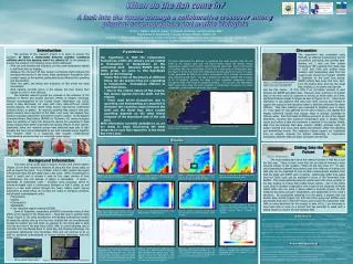
When do the fish come in? A look into the future through a collaborative crossover among physical oceanographers and marine biologists Christi J. Welter1, Scott M. Glenn2, Thomas M. Grothues3, and Kenneth W. Able3 1Department of Engineering, Colorado School of Mines, Golden, CO 2Institute of Marine and Coastal Sciences, Rutgers University, Coastal Ocean Observation Laboratory, New Brunswick, NJ 3Institute of Marine and Coastal Sciences, Rutgers University, Marine Field Station, Tuckerton, NJ Discussion Hypothesis This experiment was conducted using MATLAB, an effective programming tool for successfully processing and plotting data. Starting out, I took sea floor bottom temperature (BT) readings from glider data in 2005 and 2006 and plotted these missions with temperature data from the System-wide Monitoring Program (SWMP) in Tuckerton for the same time period. SWMP collects data every half hour, 24/7, from the Mullica River and into the Great Bay, enabling us to clearly see high tide • Our hypothesis is that the temperature fluctuations within the estuary can be related to fluctuations in temperature on the continental shelf. Between RUMFS and the COOL group, we came to this hypothesis based on the following: • Since fish arrive at the estuary at different times, we can assume they are responding to temperature fluctuations offshore to lead them there. • Due to the remote nature of the estuary, fish receive signals from the shelf, not the estuary. • These wind driven fluctuations due to upwelling and downwelling are assumed to dominate the transition region between the shelf and the Great Bay, since coastal upwelling depends on the wind driven response of the shoreward side of the cold pool. • With information currently available to us, we are ready to begin discovering the what temperature cues fish respond to in the Great Bay every year. To better understand the difficulty in predicting the exact moment that fish will arrive at the estuary each year, the figures below depict the distinct annual temperature variation from north to south along the East coast. Figure 3 shows the 10 locations that were hand picked to show this broad range of temperature data, and figure 4 shows how much the temperature changes during the course of a year. It was generated by taking sea surface temperature (SST) readings from satellite data collected during 2005. The figure displays the monthly satellite SST averages of all 10 locations, showing the range in their respective temperature cycles throughout 2005, from Arctic to equatorial climates. In conclusion, the Mid-Atlantic Bight region does show the most variability in temperature (Locations 4-7) when compared to other locations along the East coast. Figure 14. The above map shows the many locations from which data was acquired, relative to the COOL room and RUMFS. and low tide events. At first, little if no correlation seemed to exist between the SWMP and glider data. However, when zooming in to specific days in the time series as opposed to looking at whole years at a time, significant features began to appear as seen in figures 10-13. Upon closer inspection, it was apparent that data from other sources was needed to support the suspicion that estuarine water is definitely influenced by water offshore. Thus data collection was expanded to locations seen in Figure 14. First, glider ST was gathered for the same missions, and satellite SST images confirmed visually that estuary water is strongly correlated to offshore water. Data from Node B offshore proved to be one of the biggest influencers, showing that maximum temperature peak in estuary water occurs just before a high tide maximum is reached in the estuary. Finally, data from the National Data Buoy Center’s (NDBC) Ambrose Light, NY station showed how much wind speed and direction affect the upwelling and downwelling events. This expansion helped support our hypothesis from all aspects, showing the distinct relationship in temperature fluctuations between offshore water and water into the bay. Figure 3. 10 Locations along east coast with noticeable annual temperature variability Figure 4. Monthly Average SST 2005. Gliding Into the Future RIOS Research Cruise with Dr. Scott Glenn Getting ready for my first glider deployment Female blue crab Catfish caught from otter trawling Figure 15. Acoustic bioprobe Figure 16. Attachment to glider The most exciting part about this research project is that this is just the first step. There is much more that can be done to forming a more concrete answer to the question, “When do the fish come in?” To start, since temperature patterns were clearly seen from offshore to onshore, the data sets can be expanded to look at other measurements available from both the glider and SWMP, such as salinity. Additionally, glider time scales from the COOL room can be matched to those of fish movement from RUMFS. This could potentially pinpoint exactly when fish arrive, possibly to the day, leading to models that predict future activity. Also in the COOL room, there is another collaboration with a team at the University of Rhode Island (URI) who are using a device called a bioprobe (Figure 15) that measures acoustics, pressure, temperature, and acceleration in the x and y directions. By successfully attaching it to the glider, a process that has already been started (Figure 16), both the COOL group and RUMFS could acoustically track fish in both the estuary and around the continental shelf. With so many directions for this project to take off to, I am fortunate to have been able to work on a project that has potential to make such a lasting impact on marine life and mankind alike. Upwelling Figure 5. On May 13, 2006, warm shelf water covers the lower half of New Jersey. Figure 6. Seven days later on May 20, this shelf water cools off as winds from the northwest bring in cold water from offshore. Figure 7. Temperature near shore continues to drop on May 22 as winds continue to cause upwelling, bringing in cold offshore water. Figure 8. At the end of this upwelling event, shelf waters start to warm up again. Figure 9. Map of the Location of Buoy 126, courtesy of the SWMP (System-wide Monitoring Program) at the Jacques Cousteau National Estuarine Research Reserve (JCNERR) in Tuckerton. Figure 7a. A close-up of Great Bay on May 22 shows warm waters inside the bay at early morning hours of low tide flowing on to the shelf. Figure 7b. 4 hours later, high tide brings in cold offshore waters, cooling the bay off. Figure 7c. Another 4 hours later, low tide brings this cool water out, and the bay starts to warm up again. References Able, K.W., T.M. Grothues, (2006). Diversity of striped bass (Morone saxatilis) estuarine movements: synoptic examination in a passive, gated listening array. Glenn, S., R. Arnone, T. Bergmann, W.P. Bissett, M. Crowley, J. Cullen, J. Gryzmski, D. Haidvogel, J. Kohut, M. Moline, M. Oliver, C. Orrico, R. Sherrell, T. Song, A. Weidemann, R. Chant, O. Schofield, (2004). Biogeochemical impact of summertime coastal upwelling on the New Jersey Shelf, J. Geophys. Res., 109, C12S02, doi:10.1029/2003JC002265. Neuman, M., (1996). Evidence of upwelling along the New Jersey coastline and the south shore of Long Island, New York. Bull N.J. Acad. Sci. 41(1): 7-13. Rutgers University (R.U.) COOL, (2005). About Slocum Autonomous Underwater Gliders. <http://marine.rutgers.edu/cool/technology/gliders.htm> (June 7, 2006) Schofield, O., J. Kohut, D. Aragon, L. Creed, C. Haldeman, J. Kerfoot, H. Roarty, C. Jones, D. Webb, S. Glenn, (2006). Slocum gliders: Robust and ready. Webb Research Corporation, (1999). The electric glider: vehicle operation theory. < http://www.webbresearch.com/electric_glider.htm> (June 8, 2006) Acknowledgements This research project could not have been even remotely possible if it weren’t for the help of the following people, and a sincere THANK YOU is extended to them: Scott Glenn, Oscar Schofield, Ken Able, and Thomas “Motz” Grothues – for their genuine, personal, and professional guidance throughout, and for never being too busy to share their contagious passion for their research; Jen Bosch and Donglai Gong – for taking the time to share the pain and beauty of MATLAB, and for their friendship; Bob Chant and Gregg Sakowicz – for taking the time to prepare, supply and explain data for my project; Dave Aragon, Josh Graver, Chip Haldeman, John Kerfoot, Josh Kohut, Courtney Kohut, Sage Lichtenwalner, Hugh Roarty, and Arthur Yan – for representing a commendable and ideal example of sincere dedication and team work to the COOL room at Rutgers University Figure 10. The figure above shows glider surface temperature (ST) and bottom temperature (BT) related to temperature data from inside the estuary at Buoy 126 (SWMP). Looking at satellite images and time scale graphs together, BT and ST are close to the same temperature around the time of the upwelling event from May 22 – 24. Figure 11. In this figure, tide heights are shown on a time scale. Maximums represent high tide, while minimums indicate low tide events. When figures 10 and 11 are overlaid, there is a clear distinction between buoy temperature and tide height – the temperature peaks in figure 10 occur just before high tide events in figure 11. Figure 12. This time scale graph shows both wind speed and direction from May 18 – 25, 2006. Southeast wind direction during days 142 – 144 (May 21 – 23) matches southeast winds shown in the satellite images in figures 6-9. Figure 13. The map above shows the exact GPS location of the glider during this mission. The temperature scale can be matched to the BT readings in figure 10. Figure 1. The Slocum AUV ready for one of its mission in Kauai, Hawaii. Figure 2. Great Bay, Mullica River, and RUMFS in Tuckerton, NJ. Introduction • The purpose of this research project is to begin to answer the question, Is there a relationship between weather conditions offshore and in the estuary; and if so, what is it? In the attempt to answer this question, the following issues will be addressed: • Fish are cold blooded and migratory, so they need temperature signals to tell them when to migrate. • Because the cold pool off New Jersey’s continental shelf produces the strongest thermocline in the world, these temperature fluctuations have a major impact on fish activity, particularly those influenced by upwelling and downwelling. • Over the years, the timing and frequency of fish arrival has been inconsistent. • Fish tracking currently occurs in the estuary, but they receive their signals to come in from offshore. • Two separate research groups are involved in this endeavor at the Institute of Marine and Coastal Sciences (IMCS) at Rutgers University. Physical oceanographers at the Coastal Ocean Observation Lab (COOL room) in New Brunswick, NJ, work with many state-of-the-art remote sensing devices, the most recent being Slocum autonomous underwater vehicles (AUVs), or gliders. By regularly sampling New Jersey’s cold pool, gliders become more important to the COOL room every day because they measure important parameters beneath the ocean’s surface. At the Rutgers University Marine Field Station (RUMFS) in Tuckerton, NJ, marine biologists track the locations of many fish among the diverse fish population in New Jersey, helping them better understand the varying lifestyle of each species. Separately, these two research groups have gathered large sets of data annually but have not yet attempted to put their individual pieces together. This research effort is a beginning step towards collaboratively understanding and preserving our invaluable ocean waters. Results Background Information • The COOL group works daily to launch, monitor and retrieve gliders (Figure 1) from their respective missions all along the New Jersey coast, as well as around the globe. From October 2003 to date, gliders have spent 576 calendar days and 819 glider days in the water. When considering how much it would cost to operate a boat for this same amount of time (~$1000/day), the cost savings of gliders is remarkable. A glider – essentially an underwater robot – functions using buoyancy, where its volume-to-weight ratio is continuously changed so that it glides up and down in a saw tooth pattern through the ocean. Gliders collect various parameters as listed below, all of which are useful to biological, chemical, and physical oceanographers alike: • Temperature • Salinity • Chlorophyll a • Backscatter • Color dissolved organic material (CDOM) • Down at Tuckerton, researchers at RUMFS concentrate many of their efforts in the estuary in the Mullica River – Great Bay area in southern New Jersey (Figure 2). By using biotelemetry and wireless hydrophones located all along the estuary and up into the river, multiple fish are simultaneously tracked by location day and night, as opposed to only being able to track one fish at a time in the past (circa 1993). With a current sampling rate of 76.8 KHz from the Mullica down to Great Bay, fish tracking technology has progressed significantly since November 2002 and will continue to do so with an advanced understanding of remote sensing technology from the COOL room.