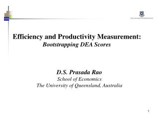
Efficiency and Productivity Measurement: Basic Concepts

1. Efficiency and Productivity Measurement:Basic Concepts D.S. Prasada Rao School of Economics The University of Queensland, Australia

2. Objectives for the Workshop • Examine the conceptual framework that underpins productivity measurement • Introduce three principal methods • Index Numbers • Data Envelopment Analysis • Stochastic Frontiers Examine these techniques, relative merits, necessary assumptions and guidelines for their applications

3. Objectives for the Workshop • Work with computer programs (we use these in the afternoon sessions) • TFPIP; EXCEL • DEAP • FRONTIER • Briefly review some case studies and real life applications • Briefly review some advanced topics on Thursday and Friday morning

4. Main ReferenceAn Introduction to Efficiency and Productivity Analysis (2nd Ed.)Coelli, Rao, O’Donnell and BatteseSpringer, 2005Supplemented with material from other published papers

5. Outline for today • Introduction • Concepts • Production Technology • Distance Functions • Output and Input Oriented distance functions • Techniques for Efficiency and Productivity Measurement: • Index Number methods

6. Introduction • Performance measurement • Productivity measures • Benchmarking performance • Mainly using partial productivity measures • Cost, revenue and profit ratios • Performance of public services and utilities • Aggregate Level • Growth in per capita income • Labour and total factor productivity growth • Sectoral performance • Labour productivity • Share in the total economy • Industry Level • Performance of firms and decision making units (DMUs) • Market and non-market goods and services • Efficiency and productivity • Banks, credit unions, manufacturing firms, agricultural farms, schools and universities, hospitals, aged care facilities, etc. • Need to use appropriate methodology to benchmark performance

7. Efficiency: • How much more can we produce with a given level of inputs? • How much input reduction is possible to produce a given level of observed output? • How much more revenue can be generated with a given level of inputs? Similarly how much reduction in input costs be achieved? • Productivity: • We wish to measure the level of output per unit of input and compare it with other firms • Partial productivity measures – output per person employed; output per hour worked; output per hectare etc. • Total factor productivity measures – Productivity measure which involves all the factors of production • More difficult to conceptualise and measure

8. Simple performance measures • Can be misleading • Consider two clothing factories (A and B) • Labour productivity could be higher in firm A – but what about use of capital and energy and materials? • Unit costs could be lower in firm B – but what if they are located in different regions and face different input prices?

9. Terminology? • The terms productivity and efficiency relate to similar (but not identical) things • Productivity = output/input • Efficiency generally relates to some form benchmark or target • A simple example – where for firm B productivity rises but efficiency falls:

10. Basic Framework: Production Technology • We assume that there is a production technology that allows transformation of a vector of inputs into a vector of outputs S = {(x,q): x can produce q}. • Technology set is assumed to satisfy some basic axioms. • It can be equivalently represented by • Output sets • Input sets • Output and input distance functions • A production function provides a relationship between the maximum feasible output (in the single output case) for a given set of input • Single output/single input; single output/multiple inputs; multi-output/multi-input

11. Output and Input sets • Output set P(x) for a given vector of inputs, x, is the set of all possible output vectors q that can be produced by x. P(x) = {q: x can produce q} = {q : (x,q)  S} • P(x) satisfies a number of intuitive properties including: nothing can be produced from x; set is closed, bounded and convex • Boundary of P(x) is the production possibility curve • An Input set L(q) can be similarly defined as set of all input vectors x that can produce q. L(q) = {x: x can produce q} = {x: (x , q)  S} • L(q) satisfies a number of important properties that include: closed and convex • Boundary of L(q) is the isoquant curve • These sets are used in defining the input and output distance functions

12. Output Distance Function • Output distance function for two vectors x (input) and q (output) vectors, the output distance function is defined as: do(x,q) = min{: (q/)P(x)} • Properties: • Non-negative • Non-decreasing in q; non-increasing in x • Linearly homogeneous in q • if q belongs to the production possibility set of x (i.e., qP(x)), then do(x,q)  1 and the distance is equal to 1 only if q is on the frontier.

13. y2 B  y2A C  A  P(x) y1A y1 0 PPC-P(x) Output Distance Function Do(x,y) The value of the distance function is equal to the ratio =0A/0B. Output-oriented Technical Efficiency Measure: TE = 0A/0B = do(x,q)

14. Input Distance Function • Input distance function for two vectors x (input) and q (output) vectors is defined as: di(x,q) = max{: (x/)L(q)} • Properties: • Non-negative • Non-decreasing in x; non-increasing in q • Linearly homogeneous in x • if x belongs to the input set of q (i.e., xL(q)), then di(x,q)  1 and the distance is equal to 1 only if x is on the frontier.

15. Input Distance Function Di(x,y The value of the distance function is equal to the ratio =0A/0B. Technical Efficiency = TE = 1/di(x,q) = OB/OA

16. Input and Output Distance Functions • What is the relationship between input and output distance functions? • If both inputs and outputs are weakly disposable, we can state that di(x,q)  1 if and only if do(x,q)  1. • If the technology exhibits global constant returns to scale then we can state that: di(x,q) = 1/do(x,q), for all x and q

17. Objectives for the firm • The production technology defines the technological constraint faced by the firm • The objective of the firm could be to maximise profit • Or minimise costs when outputs are fixed • Or maximise revenue when inputs are fixed • Or ….

18. Profit maximisation • Firms produce a vector of M outputs (q) using a vector of K inputs (x) • The production technology (set) is: • Maximum profit is defined as: where p is a vector of M output prices and w is a vector of K input prices

19. Profit maximisation Iso-profit line: q = π/p + (w/p)x q frontier Profit max x

20. Cost minimisation • The firm must produce output, q0 • Minimum cost is defined as: x1 Cost min Iso-cost line: x1 = c/w1 – (w2/w1)x2 Isoquant (q=q0) x2

21. Revenue maximisation • The firm has input allocation, x0 • Maximum revenue is defined as: y1 Revenue max Iso-revenue line: y1 = r/p1 – (p2/p1)y2 PPC (x=x0) y2

22. Short versus long run • In the long run all things can vary • In the short run some things are fixed • Cost min can be viewed as profit max in the short run when outputs are fixed • Revenue max can be viewed as profit max in the short run when inputs are fixed • One can also fix a subset of inputs (e.g., capital) and look at short run profit max or short run cost min, etc.

23. Production function Marginal product Production elasticity Scale elasticity

24. Returns to Scale • A production technology exhibits constant returns to scale (CRS) if a Z% increase in inputs results in Z% increase in outputs (ε = 1). • A production technology exhibits increasing returns to scale (IRS) if a Z% increase in inputs results in a more than Z% increase in outputs (ε > 1). • A production technology exhibits decreasing returns to scale (DRS) if a Z% increase in inputs results in a less than Z% increase in outputs (ε < 1).

25. Returns to scale q DRS CRS IRS x

26. Economies of scope • Is it less costly to produce M different products in one firm versus in M firms? • One measure of economies of scope is: • S > 0 implies economies of scope – it is better to produce the M outputs in one firm. • Other measures: • product specific measures • second derivative measures

27. Efficiency Measures • Using the distance functions defined so far, we can define: • Technical efficiency • Allocative efficiency • Economic efficiency • A firm is said to be technically efficient if it operates on the frontier of the production technology • A firm is said to be allocatively efficient if it makes efficient allocation in terms of choosing optimal input and output combinations. • A firm is said to be economically efficient if it is both technically and allocatively efficient.

28. Productivity and Efficiency Concepts • Concepts • technical efficiency • scale efficiency • allocative efficiency • cost efficiency • revenue efficiency • total factor productivity (TFP) • Brief overview of empirical methods

29. Technical Efficiency q Frontier B Output orientation: TEO=DA/DB Input orientation: TEI=EC/EA  C E   A D x

30. Scale Efficiency CRS Frontier q VRS Frontier TEVRS=DB/DA TECRS = DC/DA SE=DC/DB = TECRS/TEVRS C D    A B x

31. Allocative Efficiency AE=360/420=0.86

32. Allocative Efficiency (2) TE=400/560=0.71 AE=360/400=0.9 CE=360/560=0.64

33. Output orientated efficiency shirts C · · B D · iso-revenue line · A PPC TEO=0A/0B AEO=0B/0C RE=0A/0C =TEO×AEO 0 trousers

34. Productivity? • productivity = output/input • What to do if we have more than one input and/or output? • partial productivity measures • aggregation

35. Example • Two firms producing t-shirts using labour and capital (machines). • The partial productivity ratios conflict.

36. Total factor productivity (TFP) • Use an aggregate measure of input: • TFP = y/(a1x1+a2x2) • What should we use as the weights? – prices? • Data: Labour wage = $80 per day and • Rental price of the machines = $100 per day • Calculation: • TFPA = 200/(80×2+100×2) = 200/360 = 0.56 • TFPB = 200/(80×4+100×1) = 200/420 = 0.48 • =>A is more productive using this measure.

37. TFP decomposition • Can decompose TFP difference between 2 firms (at one point in time) into 3 types of efficiency: • technical efficiency; • allocative efficiency; and • scale efficiency. • Need to know the technology

38. TFP growth components • technical change (TC) • technical efficiency change (TEC) • scale efficiency change (SEC) • allocative efficiency change (AEC)

39. How do we measure efficiency? • Depends upon the type of data available for the measurement purpose. • Three types: • Observed input and output data for a given firm over two periods or data for a few firms at a given point of time; • Observed input and output data for a large sample of firms from a given industry (cross-sectional data) • Panel data on a cross-section of firms over time • In the first case measurement is limited to productivity measurement based on restrictive assumptions.

40. Overview of Methods • index numbers (IN) • Price and quantity index numbers used in aggregation (eg. Tornqvist, Fisher) • data envelopment analysis (DEA) • non-parametric, linear programming • stochastic frontier analysis (SFA) • parametric, econometric

41. Relative merits of Index Numbers • Advantages: • only need 2 observations • transparent and reproducible • easy to calculate • Disadvantages: • need price information • cannot decompose

42. Relative merits of Frontier Methods • DEA advantages: • no need to specify functional form or distributional forms for errors • easy to accommodate multiple outputs • easy to calculate • SFA advantages: • attempts to account for data noise • can conduct hypothesis tests