Implementing Relational Algebra: Projection
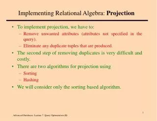
Implementing Relational Algebra: Projection. To implement projection, we have to: Remove unwanted attributes (attributes not specified in the query). Eliminate any duplicate tuples that are produced. The second step of removing duplicates is very difficult and costly.

Implementing Relational Algebra: Projection
E N D
Presentation Transcript
Implementing Relational Algebra: Projection • To implement projection, we have to: • Remove unwanted attributes (attributes not specified in the query). • Eliminate any duplicate tuples that are produced. • The second step of removing duplicates is very difficult and costly. • There are two algorithms for projection using • Sorting • Hashing • We will consider only the sorting based algorithm.
Projection operator – an example query • Consider the following query: SELECT sid, bid FROM Reserves • Assume that combined size of attributes sid and bid is 10 bytes. The result of the above query will contain 100,000 tuples and will occupy 250 pages (each page now contains 400 tuples).
Projection based on Sorting • The algorithm has the following steps: • Scan R and produce a relation with only specified attributes (discarding unwanted attributes). • Sort the above temporary relation using all the projected attributes as a key for the sorting order. • Scan the sorted temporary relation and discard duplicates by comparing adjacent tuples. • The above algorithm can be improved by combining projection with duplicate elimination. • If there are B number of buffer pages, M number of pages in relation R then the cost of projection is: • Cost of projection = M I/O, suppose that the projected relation is of size T pages, then • Cost of Sorting = 2 * T * ( log B-1 2* B) • The total cost = M + 2 * T * ( log B-1 2* B)
Projection based on Sorting … • Let us compute the cost of Projection for our example: • Cost of projection = 1000 I/O • The result of the projection will contain 100,000 tuples and will occupy 250 pages, so Let T = 250 • Let we have 20 buffer pages, so Let B = 20 • Cost of Sorting = 2 * T * ( log B-1 2 * B) = 2 * 250 * ( log 19 2 * 20) = 2 * 250 * ( log 40 / log 19) = 2 * 250 * (1.6020 / 1.2787) = 2 * 250 * ( 1.25 1) = 2 * 250 * ( 1) = 500 • The total cost = 1000 + 500 = 1500 I/Os.
Implementing Relational Algebra: Join • Consider the query: SELECT * FROM Reserves R, Sailors S WHERE R.sid = S.sid This query is translated into Reserves ⋈Sailors • Join operation is very useful and widely used in relational query processing. • Consider some terminologies for R ⋈S • Suppose that there are M pages in R, pR tuples per page, • Suppose that there are N pages in S, pS tuples per page
Simple Nested Loops Join (tuple-oriented) • For each tuple in the outer relation R, we scan the entire inner relation S: Foreach tuple r in R do Foreach tuple s in S do If ri = sj then add <r, s> to result • Cost = M + pR * M * N, where • M is the number of pages in R, • pR is the number of tuples of R per page, and • N is the number of pages in S. • Cost for our example is: • 1000 + 100 * 1000 * 500 = 50,001,000 I/Os
Simple Nested Loops Join (page-oriented) • For each page of the outer relation R, we scan the entire inner relation S: Foreach page of R do Foreach page of S do If ri = sj then add <r, s> to result, where r is in R-page and s is in S-page • Cost = M + M * N • Cost for our example is: • 1000 + 1000 * 500 = 501,000 I/Os • Which is about 100 times less than the tuple-oriented simple nested loops (SNL) join for the same example. • If smaller relation i.e. S is outer then • Cost = 500 + 500 * 1000 = 500,500 I/Os • Always use smaller relation in the outer loop
R & S Join Result Hash table for block of R (k < B-1 pages) . . . . . . . . . Output buffer Input buffer for S Block-Nested Loops Join • Use one page as an input buffer for scanning the inner S, one page as the output buffer, and use all remaining pages to hold “block” of outer R: Foreach block of B – 2 pages of R do Foreach page of S do If ri = sj then add <r, s> to result, where r is in R-page and s is in S-page
Block-Nested Loops Join … • Cost: • With Reserves (R) as outer, B = 102 pages (buffer size) • Cost = • Which is 83 times faster than that of the same example using page-oriented SNL (i.e., 501,000 I/Os) • With 100-page block of Sailors as outer • Cost = • Which is 91 times faster than that of the same example using page-oriented SNL (i.e., 500,500 I/Os)
Index-Nested Loops Join • If there is an index on one of the relations on the join attribute, we can take advantage of the index by making the indexed relation as the inner relation: Foreach tuple r in R do Foreach tuple s in S do If ri = sj then add <r, s> to result • For each tuple r ∈ R, we use the index to retrieve matching tuples of S i.e. we compare r only with tuples of S that have the same value in the join column. • Cost = M + (TN * CR), where • M is the no. of pages in R, TN is the total number of tuples in R, • TN = pR * M, where pR is the number of tuples per page in R, and • CR is the cost of identifying & retrieving matching S tuples using index • CR is given as follows: • For each tuple r ∈ R, the cost of using the index over S is about 1 for hash, 2 for B+ tree. • The cost of then retrieving S tuples depends on clustering. • Clustered index: 1 I/O, Unclustered: up to 1 I/O per matching S tuple.
Index-Nested Loops Join - Example 1 for the hash index, 1 for retrieving the only 1 possible Sailor tuple. FK PK • Reserves (R) as outer • Cost = 1000 + ((100 * 1000) * (1 + 1)) = 1000 + 200,000 = 201,000 I/Os • Which is about 2½ times faster than that of the same example using page-oriented SNL (i.e., 501,000 I/Os) • Sailors (S) as outer (Clustered index on Reserves) • Cost = 500 + ((80 * 500) * (1 + 1)) = 500 + 80,000 = 80,500 I/Os • Which is just over 6 times faster than that of the same example using page-oriented SNL (i.e., 500,500 I/Os) • Sailors (S) as outer (Unclustered index on Reserves) • Cost = 500 + ((80 * 500) * (1 + 2.5)) = 500 + 140,000 = 140,500 I/Os • Which is just over 3½ times faster than that of the same example using page-oriented SNL (i.e., 500,500 I/Os) 1 for the hash index, 1 for retrieving on average the 2½ Reserves tuples, though in only 1 page. PK FK 1 for the hash index, 1 for retrieving on average the 2½ Reserves tuples. PK FK
Implementation of Join Operator(Summary) • Simple Nested Loops (tuple-oriented) • Cost = M + pR * M * N, where • M is the number of pages in R, • pR is the number of tuples of R per page, and • N is the number of pages in S. • Simple Nested Loops (page-oriented) • Cost = M + M * N • Block Nested Loops • Cost = • where B is the total number of buffer pages. • Index Nested Loops • Cost = M + (TN * CR), where • M is the no. of pages in R, TN = pR * M, where pR is the number of tuples per page in R, and CR is the cost of identifying & retrieving matching S tuples using index