Integer Programming
Integer Programming. Integer programming is a solution method for many discrete optimization problems Programming = Planning in this context Origins go back to military logistics in WWII (1940s).


Integer Programming
E N D
Presentation Transcript
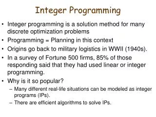
Integer Programming • Integer programming is a solution method for many discrete optimization problems • Programming = Planning in this context • Origins go back to military logistics in WWII (1940s). • In a survey of Fortune 500 firms, 85% of those responding said that they had used linear or integer programming. • Why is it so popular? • Many different real-life situations can be modeled as integer programs (IPs). • There are efficient algorithms to solve IPs.
Standard form of integer program (IP) maximizec1x1+c2x2+…+cnxn (objective function) subject to a11x1+a12x2+…+a1nxn b1 (functional constraints) a21x1+a22x2+…+a2nxn b2 …. am1x1+am2x2+…+amnxn bm x1, x2 , …, xn Z+(set constraints) Note: Can also have equality or ≥ constraint in non-standard form.
Standard form of integer program (IP) • In vector form: maximizecx (objective function) subject toAxb (functional constraints) x (set constraints) Input for IP: 1n vector c, mn matrice A, m1 vector b. Output of IP: n1 integer vector x . • Note: More often, we will consider mixed integer programs (MIP), that is, some variables are integer, the others are continuous.
Example of Integer Program(Production Planning-Furniture Manufacturer) • Technological data: Production of 1 table requires 5 ft pine, 2 ft oak, 3 hrs labor 1 chair requires 1 ft pine, 3 ft oak, 2 hrs labor 1 desk requires 9 ft pine, 4 ft oak, 5 hrs labor • Capacities for 1 week: 1500 ft pine, 1000 ft oak, 20 employees (each works 40 hrs). • Market data: • Goal: Find a production schedule for 1 week that will maximize the profit.
Production Planning-Furniture Manufacturer: modeling the problem as integer program The goal can be achieved by making appropriate decisions. First define decision variables: Let xt be the number of tables to be produced; xc be the number of chairs to be produced; xd be the number of desks to be produced. (Always define decision variables properly!)
Production Planning-Furniture Manufacturer: modeling the problem as integer program • Objective is to maximize profit: max 12xt + 5xc + 15xd • Functional Constraints capacity constraints: pine: 5xt + 1xc + 9xd 1500 oak: 2xt + 3xc + 4xd 1000 labor: 3xt + 2xc + 5xd 800 market demand constraints: tables: xt ≥ 40 chairs: xc ≥ 130 desks: xd ≥ 30 • Set Constraints xt , xc , xd Z+
Solutions to integer programs • A solution is an assignment of values to variables. • A feasible solution is an assignment of values to variables such that all the constraints are satisfied. • The objective function value of a solution is obtained by evaluating the objective function at the given point. • An optimal solution (assuming maximization) is one whose objective function value is greater than or equal to that of all other feasible solutions. • There are efficient algorithms for finding the optimal solutions of an integer program.
Next: IP modeling techniques Modeling techniques: Using binary variables Restrictions on number of options Contingent decisions Variables with k possible values Applications: Facility Location Problem Knapsack Problem
Example of IP: Facility Location • A company is thinking about building new facilities in LA and SF. • Relevant data: Total capital available for investment: $10M • Question: Which facilities should be built to maximize the total profit?
Example of IP: Facility Location • Define decision variables (i= 1, 2, 3, 4): • Then the total expected benefit: 9x1+5x2+6x3+4x4 the total capital needed: 6x1+3x2+5x3+2x4 • Summarizing, the IP model is: max9x1+5x2+6x3+4x4 s.t.6x1+3x2+5x3+2x4 10 x1, x2, x3, x4 binary ( i.e., xi{0,1} )
Knapsack problem Any IP, which has only one constraint, is referred to as a knapsack problem . • n items to be packed in a knapsack. • The knapsack can hold up to W lb of items. • Each item has weight wilb and benefit bi . • Goal: Pack the knapsack such that the total benefit is maximized.
IP model for Knapsack problem • Define decision variables (i= 1, …, n): • Then the total benefit: the total weight: • Summarizing, the IP model is: max s.t. xibinary (i= 1, …, n)
Connection between the problems • Note: The version of the facility location problem is a special case of the knapsack problem. • Important modeling skill: • Suppose you know how to model Problem A1,…,Ap; • You need to solve Problem B; • Notice the similarities between Problems Ai and B; • Build a model for Problem B, using the model for Problem Ai as a prototype.
The Facility Location Problem: adding new requirements • Extra requirement: build at most one of the two warehouses. The corresponding constraint is: x3 +x4 1 • Extra requirement: build at least one of the two factories. The corresponding constraint is: x1 +x2 ≥ 1
Modeling Technique: Restrictions on the number of options • Suppose in a certain problem, n different options are considered. For i=1,…,n • Restrictions: At least p and at most q of the options can be chosen. • The corresponding constraints are:
Modeling Technique: Contingent Decisions Back to the facility location problem. • Requirement: Can’t build a warehouse unless there is a factory in the city. The corresponding constraints are: x3 x1(LA)x4 x2(SF) • Requirement: Can’t select option 3 unless at least one of options 1 and 2 is selected. The constraint: x3 x1 + x2 • Requirement: Can’t select option 4 unless at least two of options 1, 2 and 3 are selected. The constraint: 2x4 x1 + x2 +x3
Modeling Technique: Variables with k possible values • Suppose variable y should take one of the values d1, d2, …, dk . • How to achieve that in the model? • Introduce new decision variables. For i=1,…,k, • Then we need the following constraints.
More on Integer Programming and other discrete optimization problems and techniques: • Math 4620 Linear and Nonlinear Programming • Math 4630 Discrete Modeling and Optimization