
Sorting Algorithms and Asymptotic Complexity
E N D
Presentation Transcript
Sorting and AsymptoticComplexity Lecture 14 CS2110 – Spring 2013
InsertionSort //sort a[], an array of int for (int i = 1; i < a.length; i++) { // Push a[i] down to its sorted position// in a[0..i] int temp = a[i]; int k; for (k = i; 0 < k && temp < a[k–1]; k– –) a[k] = a[k–1]; a[k] = temp; } • Many people sort cards this way • Invariant of main loop: a[0..i-1] is sorted • Works especially well when input is nearly sorted • Worst-case: O(n2) • (reverse-sorted input) • Best-case: O(n)(sorted input) • Expected case: O(n2) • Expected number of inversions: n(n–1)/4
SelectionSort //sort a[], an array of int for (int i = 1; i < a.length; i++) { int m= index of minimum of a[i..]; Swap b[i] and b[m]; } • Another common way for people to sort cards • Runtime • Worst-case O(n2) • Best-case O(n2) • Expected-case O(n2) 0 i length a sorted, smaller values larger values Each iteration, swap min value of this section into a[i]
Divide & Conquer? It often pays to • Break the problem into smaller subproblems, • Solve the subproblems separately, and then • Assemble a final solution This technique is called divide-and-conquer • Caveat: It won’t help unless the partitioning and assembly processes are inexpensive Can we apply this approach to sorting?
MergeSort • Quintessential divide-and-conquer algorithm • Divide array into equal parts, sort each part, then merge • Questions: • Q1: How do we divide array into two equal parts? A1: Find middle index: a.length/2 • Q2: How do we sort the parts? A2: Call MergeSort recursively! • Q3: How do we merge the sorted subarrays? A3: Write some (easy) code
Merging Sorted Arrays A and B into C i Picture shows situation after copying{4, 7} from A and {1, 3, 4, 6} from B into C 4 7 7 8 9 k A[0..i-1] and B[0..j-1] have been copied into C[0..k-1]. C[0..k-1] is sorted. Next, put a[i] in c[k], because a[i] < b[j]. Then increase k and i. Array A j C: merged array 1 3 4 6 8 1 3 4 4 6 7 Array B
Merging Sorted Arrays A and B into C • Create array C of size: size of A+ size of B • i= 0; j= 0; k= 0; // initially, nothing copied • Copy smaller of A[i]and B[j] into C[k] • Increment i or j, whichever one was used, and k • When either A or Bbecomes empty, copy remaining elements from the other array (B or A, respectively) into C This tells what has been done so far: A[0..i-1] and B[0..j-1] have been placed in C[0..k-1]. C[0..k-1] is sorted.
MergeSort Analysis Outline (code on website) • Split array into two halves • Recursively sort each half • Merge two halves • Merge: combine two sorted arrays into one sorted array • Rule: always choose smallest item • Time: O(n) where n is the total size of the two arrays • Runtime recurrence • T(n): time to sort array of size nT(1) = 1 • T(n) = 2T(n/2) + O(n) • Can show by induction that T(n) is O(n log n) • Alternatively, can see that T(n) is O(n log n) by looking at tree of recursive calls
MergeSort Notes • Asymptotic complexity: O(n log n) Much faster than O(n2) • Disadvantage • Need extra storage for temporary arrays • In practice, can be a disadvantage, even though MergeSortis asymptotically optimal for sorting • Can do MergeSortin place, but very tricky (and slows execution significantly) • Good sorting algorithms that do not use so much extra storage? Yes: QuickSort
QuickSort IdeaTo sort b[h..k], which has an arbitrary value x in b[h]: first swap array values around until b[h..k] looks like this: x is called the pivot h h+1 k h j k x ? <= x x >= x • Then sort b[h..j-1] and b[j+1..k] —how do you do that? • Recursively!
QuickSort 4 5 14 19 pivot 2031 24 19 45 56 4 65 5 72 14 99 partition j 19 4 5 14 20 31 24455665 72 99 Not yet sorted Not yet sorted QuickSort 2024 31 45 56 65 72 99 sorted
In-Place Partitioning • On the previous slide we just moved the items to partition them • But in fact this would require an extra array to copy them into • Developer of QuickSort came up with a better idea • In place partitioning cleverly splits the data in place
In-Place Partitioning • Choosing pivot • Ideal pivot: the median, since it splits array in half • Computing median of unsorted array is O(n), quite complicated • Popular heuristics: Use • first array value (not good) • middle array value • median of first, middle, last, values GOOD! • Choose a random element Key issues • How to choose a pivot? • How to partition array in place? Partitioning in place • Takes O(n) time (next slide) • Requires no extra space
In-Place Partitioning Change b[h..k]from this: to this by repeatedlyswapping array elements: b h h+1 k h j k h j t k x ? <= x x >= x <= x x ? >= x b Do it one swap at a time, keeping the array looking like this. At each step, swap b[j+1] with something b Start with: j= h; t= k;
In-Place Partitioning Initially, with j = h and t = k, this diagram looks like the start diagram h j t k <= x x ? >= x j= h; t= k; while (j < t) { if (b[j+1] <= x) { Swap b[j+1] and b[j]; j= j+1; } else { Swap b[j+1] and b[t]; t= t-1; } } Terminates when j = t, so the “?” segment is empty, so diagram looks like result diagram b
In-Place Partitioning • How can we move all the blues to the left of all the reds? • Keep two indices, LEFT and RIGHT • Initialize LEFT at start of array and RIGHT at end of array • Invariant: all elements to left of LEFT are blue all elements to right of RIGHT are red • Keep advancing indices until they pass, maintaining invariant
swap swap swap Now neither LEFT nor RIGHT can advance and maintain invariant. We can swap red and blue pointed to by LEFT and RIGHT indices. After swap, indices can continue to advance until next conflict.
Once indices cross, partitioning is done • If you replace blue with ≤ p and red with ≥ p, this isexactly what we need for QuickSort partitioning • Notice that after partitioning, array is partially sorted • Recursive calls on partitioned subarrays will sort subarrays • No need to copy/move arrays, since we partitioned in place
QuickSort procedure /** Sort b[h..k]. */ publicstaticvoid QS(int[] b, int h, int k) { if (b[h..k] has < 2 elements) return; int j= partition(b, h, k); // We know b[h..j–1] <= b[j] <= b[j+1..k] // So we need to sort b[h..j-1] and b[j+1..k] QS(b, h, j-1); QS(b, j+1, k); } Base case Function does the partition algorithm and returns position j of pivot
QuickSort versus MergeSort /** Sort b[h..k] */ publicstaticvoid MS (int[] b, int h, int k) { if (k – h < 1) return; MS(b, h, (h+k)/2); MS(b, (h+k)/2 + 1, k); merge(b, h, (h+k)/2, k); } /** Sort b[h..k] */ publicstaticvoid QS (int[] b, int h, int k) { if (k – h < 1) return; int j= partition(b, h, k); QS(b, h, j-1); QS(b, j+1, k); } One processes the array then recurses. One recurses then processes the array.
p > p QuickSort Analysis Runtime analysis (worst-case) • Partition can produce this: • Runtime recurrence: T(n) = T(n–1) + n • Can be solved to show worst-case T(n) is O(n2) • Space can be O(n) —max depth of recursion Runtime analysis (expected-case) • More complex recurrence • Can be solved to show expected T(n) is O(n log n) Improve constant factor by avoiding QuickSort on small sets • Use InsertionSort(for example) for sets of size, say, ≤ 9 • Definition of small depends on language, machine, etc.
Sorting Algorithm Summary Why so many? Do computer scientists have some kind of sorting fetish or what? Stable sorts: Ins, Sel, Mer Worst-case O(n log n): Mer, Hea Expected O(n log n): Mer, Hea, Qui Best for nearly-sorted sets: Ins No extra space: Ins, Sel, Hea Fastest in practice: Qui Least data movement: Sel We discussed • InsertionSort • SelectionSort • MergeSort • QuickSort Other sorting algorithms • HeapSort(will revisit) • ShellSort(in text) • BubbleSort(nice name) • RadixSort • BinSort • CountingSort
Lower Bound for Comparison Sorting Goal: Determine minimum time required to sort n items Note: we want worst-case, not best-case time • Best-case doesn’t tell us much. E.g. Insertion Sort takes O(n) time on already-sorted input • Want to know worst-case time for best possible algorithm • How can we prove anything about the best possible algorithm? • Want to find characteristics that are common to all sorting algorithms • Limit attention to comparison-based algorithms and try to count number of comparisons
Comparison Trees • Comparison-based algorithms make decisions based on comparison of data elements • Gives a comparison tree • If algorithm fails to terminate for some input, comparison tree is infinite • Height of comparison tree represents worst-case number of comparisons for that algorithm • Can show: Anycorrect comparison-based algorithm must make at least n log n comparisons in the worst case a[i] < a[j] yes no
Lower Bound for Comparison Sorting • Say we have a correct comparison-based algorithm • Suppose we want to sort the elements in an array b[] • Assume the elements of b[]are distinct • Any permutation of the elements is initially possible • When done, b[]is sorted • But the algorithm could not have taken the same path in the comparison tree on different input permutations
Lower Bound for Comparison Sorting How many input permutations are possible? n! ~ 2n log n For a comparison-based sorting algorithm to be correct, it must have at least that many leaves in its comparison tree To have at least n! ~ 2n log n leaves, it must have height at least n log n (since it is only binary branching, the number of nodes at most doubles at every depth) Therefore its longest path must be of length at least n log n, and that it its worst-case running time
java.lang.Comparable<T> Interface • public int compareTo(T x); • Return a negative, zero, or positive value • negative if this is before x • 0 if this.equals(x) • positive if this is after x • Many classes implement Comparable • String, Double, Integer, Character, Date, … • Class implements Comparable? Its method compareTois considered to define that class’s natural ordering • Comparison-based sorting methods should work with Comparable for maximum generality