Grid Computing
Grid Computing. 李孝治. Outline. Introduction to Grid Computing Standards for Grid Computing Scheduling for Grid Systems. 1. Introduction to Grid Computing. “Grid Services for Distributed System Integration” Foster , Kesselman, Nick, and Tuecke, IEEE Computer, June 2002.


Grid Computing
E N D
Presentation Transcript
Grid Computing 李孝治
Outline • Introduction to Grid Computing • Standards for Grid Computing • Scheduling for Grid Systems
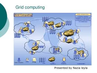
1. Introduction to Grid Computing • “Grid Services for Distributed System Integration” • Foster, Kesselman, Nick, and Tuecke, IEEE Computer, June 2002. • Grid technologies and infrastructures support the sharing and coordinated use of diverse resources in dynamic, distributedvirtualorganizations (VO)
VirtualOrganizations (VO) include • Creation ofvirtual computing systems • Geographically distributed components operated by distinct organizations with differing policies, • Sufficiently integrated to deliver the desired QoS. • Resources: • Computational devices, • Networks, • Online instruments, • Storage archives, • etc.
“What is Grid?A Three Point Checklist” • http://www-ip.mcs.anl.gov/~foster/Articles/WhatIsTheGrid.pdf 1) coordinatesresources that are not subject to centralized control … 2)… using standard, open, general-purpose protocols and interfaces… 3)… to deliver nontrivial 重要 qualities of service.
“The Anatomy 解剖of the Grid” • http://www.globus.org/research/papers/anatomy.pdf • “Grid” computing has emerged as an important new field, distinguished fromconventional distributed computing by its focus on • large-scale resource sharing, • innovative applications, • and, in some cases, high-performance orientation.
Grid Applications • Application service providers • Storage service providers • Consultants engaged by a car manufacturer to perform scenario evaluation during planning for a new factory • Members of an industrial consortium 財團bidding on a new aircraft • A crisismanagementteam and the databases and simulation systems that they use to plan a response to an emergency situation • Members of a large, international, multiyear high-energy physics collaboration
2. Standards for Grid Computing • A de facto standard for Grid systems: OGSA (Open Grid Services Architecture) Globus Toolkit version 3 (GT3) • Defines a uniform exposed servicesemantics(the Grid service); • Defines standard mechanisms for creating, naming, and discovering transient Grid service instances; • Provides location transparency and multiple protocol bindings for service instances; • Supports integration with underlying native platform facilities.
Core • Grid service interfaces • Base • resource management • data transfer • information services • reservation • monitoring • Data • data management • Grid • workload management • diagnostics
Figure 2. Three different VO structures (1) A simple hosting environment A set of resources located within a single administrative domain (2) A virtual hosting environment A set of resources span two B2B domains (3) Collective services a set of resources span two E2E domains
3. Scheduling in Grid Systems • “Scheduling strategies for mixed data and task parallelism on heterogeneous clusters and grids” • O. Beaumont, A. Legrand, and Y. Robert • Proceedings of the Eleventh Euromicro Conference on Parallel-Distributed and Network-Based Processing (Euro-PDP’03)
The complex application consists of a suite ofidentical, independentproblems to be solved. • Each problem consists of a set of tasks. • There are dependences (precedence constraints) between these tasks. • Fork graph (task graph) • A probleminstance: • e.g. a loop iteration of 4 tasks • Operates on different data
Platform graph • E.g. 4 resources and 5 communication links • Both with different rates • Master node: an initial node • The question for the master is to decide • which tasks to execute itself, • and how many tasks to forward to each of its neighbors. • Each neighbor faces in turn the same dilemma.
Due to heterogeneity, the neighbors may receive different amounts of work (maybe none for some of them). • Because the problems are independent, their execution can be pipelined. • At a given time-step, different processors may well compute different tasks belonging to different problem instances.
Objective • To determine the optimalsteady statescheduling policy for each processor • That is, the fraction of time spent computing, and the fraction of time spent sending or receiving each type of tasks along each communication link, so that the (averaged) overall number of problems processed at each time-step is maximum.
The model • The application • Let P(1), P(2), …, P(n) be the nproblems to solve, where n is large. • Each problem P(m) corresponds to a copyG(m) = (V(m), E(m)) of the same task graph(V, E). • The number |V| of nodes in V is the number of task types. • In the example of Figure 1, there are four task types, denoted as T1, T2, T3 and T4. • Overall, there are n * |V| tasks to process, since there are n copies of each task type.
The architecture • The target heterogeneous platform is represented by a directed graph, the platform graph. • There are pnodesP1, P2, … , Pp that represent the processors. • In the example of Figure 2 there are four processors, hence p = 4. • Each edge represents a physical interconnection. • Each edge eij : PiPj is labeled by a valuecij which represents the time to transfer a message ofunit length between Pi and Pj, in either direction. • We assume a full overlap, single-portoperation mode, where a processor node can simultaneouslyreceive data from one of its neighbor, perform some (independent) computation, and send data to one of its neighbor.
Execution time • ProcessorPi requires wi,ktimeunits to process a task of typeTk. • Assume that wi,k = wiδk, where wiis the inverse of the relative speed of processor Pi, and δk the weight of task Tk. • Communication time • Each edgeek,l: TkTl in the task graph is weighted by a communicationcostdatak,lthat depends on the tasks Tk and Tl. It corresponds to the amount of dataoutput by Tk and required as input to Tl. • The time to transfer the data from Pi to Pj is equal to datak,l ci,j
Steady-state equations • The (average) fractionof time spent each time-unit by Pi to send to Pj data involved by the edgeek,l. s(PiPj, ek,l) = sent(PiPj, ek,l) (datak,l ci,j) (1) where sent(PiPj, ek,l) denotes the (fractional) number offiles sent per time-unit • The (average) fraction of time spent each time-unit by Pi to process tasks of typeTk: α(Pi, Tk) = cons(Pi, Tk) wi,k(2) where cons(Pi, Tk) denotes the (fractional) number oftasks of type Tk processed per time unit by processor Pi.
Activities during one time-unit • One-port model for outgoing communications • One-port model for incoming communications
Theorem 1.The solution to the previous linearprogramming problem provides the optimal solution to SSSP(G).
Conclusions • We have shown how to determine the beststeady statescheduling strategy for a general task graph and for a general platform graph, using a linear programming approach. • This work can be extended in the following twodirections: • On the theoretical side, we could try to solve the problem of maximizing the number of tasks that can be executed within K time-steps, where K is a given time bound. [Initialization phase] • On the practical side, we need to run actual experiments rather than simulations. End
Other scheduling for Grid systems • Local grid scheduling techniques using performance predictionSpooner, D.P.; Jarvis, S.A.; Cao, J.; Saini, S.; Nudd, G.R.;Computers and Digital Techniques, IEE Proceedings- , Volume: 150 Issue: 2 , March 2003 • Ant algorithm-based task scheduling in grid computingZhihong Xu; Xiangdan Hou; Jizhou Sun;Electrical and Computer Engineering, 2003. IEEE CCECE 2003. Canadian Conference on , Volume: 2 , May 4-7, 2003
Near-optimal dynamic task scheduling of independent coarse-grained tasks onto a computational gridFujimoto, N.; Hagihara, K.;Parallel Processing, 2003. Proceedings. 2003 International Conference on , 6-9 Oct. 2003 • Scheduling in a grid computing environment using genetic algorithmsDi Martino, V.; Mililotti, M.;Parallel and Distributed Processing Symposium., Proceedings International, IPDPS 2002, Abstracts and CD-ROM , 15-19 April 2002 End