Download
1 / 17
260 likes | 844 Vues
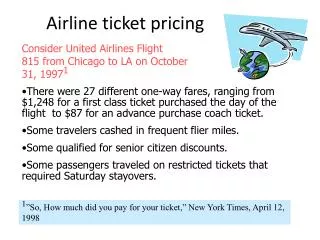
Airline ticket pricing. Consider United Airlines Flight 815 from Chicago to LA on October 31, 1997 1 There were 27 different one-way fares, ranging from $1,248 for a first class ticket purchased the day of the flight to $87 for an advance purchase coach ticket.

E N D
Airline ticket pricing • Consider United Airlines Flight 815 from Chicago to LA on October 31, 19971 • There were 27 different one-way fares, ranging from $1,248 for a first class ticket purchased the day of the flight to $87 for an advance purchase coach ticket. • Some travelers cashed in frequent flier miles. • Some qualified for senior citizen discounts. • Some passengers traveled on restricted tickets that required Saturday stayovers. 1”So, How much did you pay for your ticket,” New York Times, April 12, 1998
Assumptions • You are a manager for a regional airline offering non-stop service between Houston, TX and Orlando, FL. • Your airline makes one departure from each city per day (2 flights total). • One rival airline offers non-stop service on this route. • We ignore first class service and focus on the demand for coach-class travel.
The demand function Q = f(P, PO, Y) [1] [3.1] can be read as follows:The number of your airline’s coach seats sold per flight (Q) is a function of the your airline’s coach fare (P), its rival’s fare (PO), and income in the region (Y) Your forecasting unit has estimated the following demand function: Q = 25 + 3Y + PO – 2P [2]
Effect of changes in the explanatory variables Q is the dependent variable; P, PO, and Y are the independent or explanatory variables. • For each one point increase in the income index (Y), 3 additional seats will be sold, ceteris paribus. • For each $10 increase in the airline’s fare, 20 fewer seats will be sold, ceteris paribus. • For each $10 increase in the competitor’s fare, 10 additional seats will be sold, ceteris paribus.
The multivariable regression model How did the Forecasting Unit estimate that equation? Multivariable regression is a technique that allows for more than one explanatory variable.
Model specification Suppose that airline ticket sales are a function of three variables, that is: Q = f(P, PO, Y) [3.1] Qis the airline’s coach seats sold per flight; P is the fare; P0 is the rival’s fare; and Y is a regional income index. Our regression specification can be written as follows:
Estimating multivariable regression models using OLS Let: Yi = 0 + 1X1i+ 2X2i + i Computer algorithms find the ’s that minimize the sum of the squared residuals:
Results of the regression Our equation is estimated as follows:
The F test The F test provides another “goodness of fit” criterion for our regression equation. The F test is a test of joint significance of the estimated regression coefficients. The F statistic is computed as follows: Where K - 1 is degrees of freedom in the numerator and n – K is degrees of freedom in the denominator
We set up the following null hypothesis an alternative hypothesis: H0 : 1 = 2 = 3 = 0 HA: H0 is not true We adhere to the following decision rule: Reject H0 if F > FC, where FC is the critical value of F at the level of significance selected by the forecaster. Suppose we select the 5 percent significance level. The critical value of F (3 degrees of freedom in the numerator and 12 degrees of freedom in the denominator) is 3.49. Thus we can reject the null hypothesis since 13.9 > 3.49.
Example: The Demand for Coal COAL = 12,262 + 92.43FIS + 118.57FEU -48.90PCOAL + 118.91PGAS • COAL is monthly demand for bituminous coal (in tons) • FIS is the Federal Reserve Board Index of Iron and Steel production. • FEU the FED Index of Utility Production. • PCOAL is a wholesale price index for coal. • PGAS is a wholesale price index for naturalgas. Source: Pyndyck and Rubinfeld (1998), p. 218.