Noise, Information Theory, and Entropy
440 likes | 1.94k Vues
Noise, Information Theory, and Entropy. CS414 – Spring 2007 By Roger Cheng (Huffman coding slides courtesy of Brian Bailey). Why study noise?. It’s present in all systems of interest, and we have to deal with it By knowing its characteristics, we can fight it better

Noise, Information Theory, and Entropy
E N D
Presentation Transcript
Noise, Information Theory, and Entropy CS414 – Spring 2007 By Roger Cheng (Huffman coding slides courtesy of Brian Bailey)
Why study noise? • It’s present in all systems of interest, and we have to deal with it • By knowing its characteristics, we can fight it better • Create models to evaluate analytically
Communication system abstraction Information source Encoder Modulator Sender side Channel Receiver side Decoder Demodulator Output signal
The additive noise channel • Transmitted signal s(t) is corrupted by noise source n(t), and the resulting received signal is r(t) • Noise could result form many sources, including electronic components and transmission interference s(t) + r(t) n(t)
Random processes • A random variable is the result of a single measurement • A random process is a indexed collection of random variables, or equivalently a non-deterministic signal that can be described by a probability distribution • Noise can be modeled as a random process
WGN (White Gaussian Noise) • Properties • At each time instant t = t0, the value of n(t) is normally distributed with mean 0, variance σ2 (ie E[n(t0)] = 0, E[n(t0)2] = σ2) • At any two different time instants, the values of n(t) are uncorrelated (ie E[n(t0)n(tk)] = 0) • The power spectral density of n(t) has equal power in all frequency bands
WGN continued • When an additive noise channel has a white Gaussian noise source, we call it an AWGN channel • Most frequently used model in communications • Reasons why we use this model • It’s easy to understand and compute • It applies to a broad class of physical channels
Signal energy and power • Energy is defined as • Power is defined as • Most signals are either finite energy and zero power, or infinite energy and finite power • Noise power is hard to compute in time domain • Power of WGN is its variance σ2
Signal to Noise Ratio (SNR) • Defined as the ratio of signal power to the noise power corrupting the signal • Usually more practical to measure SNR on a dB scale • Obviously, want as high an SNR as possible
Original sound file is CD quality (16 bit, 44.1 kHz sampling rate) SNR example - Audio Original 40 dB 20 dB 10 dB
Analog vs. Digital • Analog system • Any amount of noise will create distortion at the output • Digital system • A relatively small amount of noise will cause no harm at all • Too much noise will make decoding of received signal impossible • Both - Goal is to limit effects of noise to a manageable/satisfactory amount
Information theory and entropy • Information theory tries to solve the problem of communicating as much data as possible over a noisy channel • Measure of data is entropy • Claude Shannon first demonstrated that reliable communication over a noisy channel is possible (jump-started digital age)
Entropy definitions • Shannon entropy • Binary entropy formula • Differential entropy
Properties of entropy • Can be defined as the expectation of log p(x) (ie H(X) = E[-log p(x)]) • Is not a function of a variable’s values, is a function of the variable’s probabilities • Usually measured in “bits” (using logs of base 2) or “nats” (using logs of base e) • Maximized when all values are equally likely (ie uniform distribution) • Equal to 0 when only one value is possible • Cannot be negative
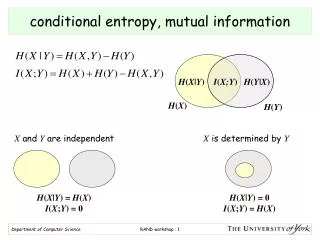
Joint and conditional entropy • Joint entropy is the entropy of the pairing (X,Y) • Conditional entropy is the entropy of X if the value of Y was known • Relationship between the two
Mutual information • Mutual information is how much information about X can be obtained by observing Y
Mathematical model of a channel • Assume that our input to the channel is X, and the output is Y • Then the characteristics of the channel can be defined by its conditional probability distribution p(y|x)
Channel capacity and rate • Channel capacity is defined as the maximum possible value of the mutual information • We choose the best f(x) to maximize C • For any rate R < C, we can transmit information with arbitrarily small probability of error
Binary symmetric channel • Correct bit transmitted with probability 1-p • Wrong bit transmitted with probability p • Sometimes called “cross-over probability” • Capacity C = 1 - H(p,1-p)
Binary erasure channel • Correct bit transmitted with probability 1-p • “Erasure” transmitted with probability p • Capacity C = 1 - p
Coding theory • Information theory only gives us an upper bound on communication rate • Need to use coding theory to find a practical method to achieve a high rate • 2 types • Source coding - Compress source data to a smaller size • Channel coding - Adds redundancy bits to make transmission across noisy channel more robust
Source-channel separation theorem • Shannon showed that when dealing with one transmitter and one receiver, we can break up source coding and channel coding into separate steps without loss of optimality • Does not apply when there are multiple transmitters and/or receivers • Need to use network information theory principles in those cases
Huffman Encoding • Use probability distribution to determine how many bits to use for each symbol • higher-frequency assigned shorter codes • entropy-based, block-variable coding scheme
Huffman Encoding • Produces a code which uses a minimum number of bits to represent each symbol • cannot represent same sequence using fewer real bits per symbol when using code words • optimal when using code words, but this may differ slightly from the theoretical lower limit • Build Huffman tree to assign codes
Informal Problem Description • Given a set of symbols from an alphabet and their probability distribution • assumes distribution is known and stable • Find a prefix free binary code with minimum weighted path length • prefix free means no codeword is a prefix of any other codeword
Huffman Algorithm • Construct a binary tree of codes • leaf nodes represent symbols to encode • interior nodes represent cumulative probability • edges assigned 0 or 1 output code • Construct the tree bottom-up • connect the two nodes with the lowest probability until no more nodes to connect
Huffman Example • Construct the Huffman coding tree (in class)
Lowest probability symbol is always furthest from root Assignment of 0/1 to children edges arbitrary other solutions possible; lengths remain the same If two nodes have equal probability, can select any two Notes prefix free code O(nlgn) complexity Characteristics of Solution
Encode “BEAD” 001011011 Decode “0101100” Example Encoding/Decoding
Entropy (Theoretical Limit) = -.25 * log2 .25 + -.30 * log2 .30 + -.12 * log2 .12 + -.15 * log2 .15 + -.18 * log2 .18 H = 2.24 bits
Average Codeword Length = .25(2) +.30(2) +.12(3) +.15(3) +.18(2) L = 2.27 bits
Code Length Relative to Entropy • Huffman reaches entropy limit when all probabilities are negative powers of 2 • i.e., 1/2; 1/4; 1/8; 1/16; etc. • H <= Code Length <= H + 1
H = -.01*log2.01 + -.99*log2.99 = .08 L = .01(1) +.99(1) = 1 Example
Limitations • Diverges from lower limit when probability of a particular symbol becomes high • always uses an integral number of bits • Must send code book with the data • lowers overall efficiency • Must determine frequency distribution • must remain stable over the data set