Spatial Statistics I
Spatial Statistics I. RESM 575 Spring 2011 Lecture 10. Spatial Statistics. Measuring geographic distributions Testing statistical significance Identifying patterns. Measuring geographic distributions. Identify spatial characteristics of a distribution Where is the center?

Spatial Statistics I
E N D
Presentation Transcript
Spatial Statistics I RESM 575 Spring 2011 Lecture 10
Spatial Statistics Measuring geographic distributions Testing statistical significance Identifying patterns
Measuring geographic distributions Identify spatial characteristics of a distribution • Where is the center? • What feature is most central? • How are features dispersed around the center?
Where is the center? • Mean Center tool • Computes the average X and Y coordinates of all features • Creates a new point feature
Mean center tool • More common use: • To compare distributions of different types of features or to find the center of features based on an attribute value
What is the most central feature? • Central feature tool • Identifies the most centrally located feature • Feature having the lowest total distance to all other features
What is the most central feature? • More interestingly is by adding a weight in the analysis such as population • We are now finding not just which site is most central but which is the most accessible to the greatest number of people.
Measuring feature distribution • Standard distance tool • Measures distribution of features around the mean • Result is a summary statistic representing distance • If circle is large, incidents are widespread • If small, incidents are more localized
Distributional trends • Directional distribution (standard ellipse) tool • Identify spatial trends in the distribution of features • Uses • Compare distributions • Examine different time periods • Show compactness and orientation
Testing statistical significance • The next section of identifying patterns or later spatial relationships allows us to perform significance tests on the results before accepting them
Using significance tests with spatial data • Spatial data contradicts some of the assumptions of inferential statistics • You need to be aware of these limitations!
Assumptions • Testing a random sample • With GIS data in a database you may not know if the data was randomly sampled • How large the sample is in relation to the population? • Even with randomness assumed, spatial data often violates the independence of observations in a sample Spatial data is rarely evenly distributed across a region
For spatial pattern analysis… • The null hypothesis is that features are evenly distributed across the study area • Hard to imagine this being true • You have to make one of two common sampling assumptions: randomization or normalization
Identifying Patterns • Why study patterns? Range from completely clustered to completely dispersed
Identifying patterns (applications) Forestry applications USFS may measure the pattern of clear cuts to ensure sufficient contiguous forest habitat remaining Agency may allow a level of clustering of clear cuts and then make sure it is not exceeded Wildlife studies if population is dispersed then species can live in a wide range of habitats, if clustered then it has very specific habitat requirements
Goal for analyzing spatial patterns • Are there underlying spatial processes influencing the locations of our features? • Are our features randomly located throughout the study area, or are they displaying a clustering or dispersed pattern?
Approaches for analyzing spatial patterns • Approach #1 Global calculations • Identifies overall patterns or trends in the data • Effective for complex messy data • Interested in broad overall results • Work by comparing feature locations and/or attributes to a theoretical random distribution to determine if you have statistically significant clustering or dispersion
Analyzing spatial patterns • Can be found with the Average Nearest Neighbor which does not require specifying an attribute, or • If based on an attribute we can test for Spatial autocorrelation using the (Moran’s I) tool • Things that are closer are more alike than things that are not • Measures similarity of neighboring features • Identifies if features are clustered or dispersed
Global SA interpretation • I > 0 positive spatial autocorrelation • I < 0 negative spatial autocorrelation The more positive or more negative, the greater amount of spatial autocorrelation
2nd Approach • Local calculations • Identify the extent and locations of clustering • Answer where do we have spatial clustering • Process every feature within the context of its neighboring features in order to determine whether it represents a spatial outlier, or if part of a statistically significant spatial cluster
Locate the hot spots • This is a local question that requires a hot spot analysis (Getis-Ord Gi*) tool • Indicates the extent to which each feature is surrounded by similarly high or low values • Where do features with similar attribute values cluster spatially together
Getis-Ord Gi* tool • Identifies where clustering occurs in both high and low values • Calculates a Z score for each feature • High Z = hot spot (when a feature has a high value and it is surrounded by other features with high values) • Low Z = cold spot (when we have features with low values surrounded by other features with low values)
Notes on the Z score • Z score is a measure of standard deviation • It is a reference value that’s associated with a standard normal distribution • A very high or low Z score would be found in the tails
More notes on Z score • A very high or low Z score means that the pattern deviates significantly from a hypothetical random pattern • For example, when using a 95% CI, Z scores are -1.96 and +1.96 • If Z is between these -1.96 and +1.96 you can’t reject the null • You are seeing one version of a random pattern • If very high or low (ie -2.5 or +5.4) you have a pattern that’s too unusual to be a pattern of random choice so we reject the null hypoth REMEMBER: The null hypothesis is that features are evenly distributed across the study area
Reference • Mitchell, A. 2005. ESRI Guide to GIS Analysis, Volume 2. ESRI press, Redlands, CA. • ArcGIS 10 Help