Definitions
In statistics, a hypothesis is a claim or statement about a property of a population. A hypothesis test is a standard procedure for testing a claim about a property of a population. Definitions. We will study hypothesis testing for population proportion p population mean

Definitions
E N D
Presentation Transcript
In statistics, a hypothesis is a claim or statement about a property of a population. A hypothesis test is a standard procedure for testing a claim about a property of a population. Definitions
We will study hypothesis testing for population proportion p population mean population standard deviation Main Objectives
Example Claim: the XSORT method of gender selection increases the likelihood of having a baby girl. This is a claim about proportion (of girls) To test this claim 14 couples (volunteers) were subject to XSORT treatment. If 6 or 7 or 8 have girls, the method probably doesnot increase the likelihood of a girl. If 13 or 14 couples have girls, the method is probably increases the likelihood of a girl.
If, under a given assumption, the probability of a particular observed event is exceptionally small, we conclude that the assumption is probably not correct. Rare Event Rule for Inferential Statistics
The null hypothesis (denoted by H0) is a statement that the value of a population parameter (such as proportion, mean, or standard deviation) is equalto some claimed value. We test the null hypothesis directly. Either reject H0 or fail to reject H0 (in other words, accept H0 ). Null Hypothesis: H0
The alternative hypothesis (denoted by H1) is the statement that the parameter has a value that somehow differs from the null hypothesis. The symbolic form of the alternative hypothesis must use one of these symbols: , <, >. (not equal, less than, greater than) Alternative Hypothesis: H1
Example 1 Claim: the XSORT method of gender selection increases the likelihood of having a baby girl. We express this claim in symbolic form: p>0.5 (here p denotes the proportion of baby girls) Null hypothesis must say “equal to”, so H0 : p=0.5 Alternative hypothesis must express difference: H1 : p>0.5 Original claim is now the alternative hypothesis
Example 1 (continued) We always test the null hypothesis. If we reject the null hypothesis, then the original clam is accepted. Final conclusion would be: XSORT method increases the likelihood of having a baby girl. If we fail to reject the null hypothesis, then the original clam is rejected. Final conclusion would be: XSORT method does not increase the likelihood of having a baby girl.
Example 2 Claim: for couples using the XSORT method the likelihood of having a baby girl is 50% Express this claim in symbolic form: p=0.5 (again p denotes the proportion of baby girls) Null hypothesis must say “equal to”, so H0 : p=0.5 Alternative hypothesis must express difference: H1 : p0.5 Original claim is now the null hypothesis
Example 2 (continued) If we reject the null hypothesis, then the original clam is rejected. Final conclusion would be: for couples using the XSORT, the likelihood of having a baby girl is not 0.5 If we fail to reject the null hypothesis, then the original clam is accepted. Final conclusion would be: for couples using the XSORTthe likelihood of having a baby girl is indeed equal to 0.5
Example 3 Claim: for couples using the XSORT method the likelihood of having a baby girl is at least 0.5 Express this claim in symbolic form: p≥0.5 (again p denotes the proportion of baby girls) Null hypothesis must say “equal to”, so H0 : p=0.5 (this agrees with the claim!) Alternative hypothesis must express difference: H1 : p<0.5 Original claim is now the null hypothesis
Example 3 (continued) If we reject the null hypothesis, then the original clam is rejected. Final conclusion would be: for couples using the XSORT, the likelihood of having a baby girl is less 0.5 If we fail to reject the null hypothesis, then the original clam is accepted. Final conclusion would be: for couples using the XSORTthe likelihood of having a baby girl is indeed at least 0.5
General rules: • If the null hypothesis is rejected, the alternative hypothesis is accepted. • If the null hypothesis is accepted, the alternative hypothesis is rejected. • Acceptance or rejection of the null hypothesis is an initial conclusion. • Always state the final conclusion expressed in terms of the original claim, not in terms of the null hypothesis or the alternative hypothesis.
A Type I error is the mistake of rejecting the null hypothesis when it is actually true. The symbol (alpha) is used to represent the probability of a type I error. Type I Error
A Type II error is the mistake of accepting the null hypothesis when it is actually false. The symbol (beta) is used to represent the probability of a type II error. Type II Error
Claim: a new medicine has a greater success rate, p>p0, than the old (existing) one. Null hypothesis: H0 : p=p0 Alternative hypothesis: H1 : p>p0(agrees with the original claim) Example
Type I error: the null hypothesis is true, but we reject it => we accept the claim, hence we adopt the new (inefficient, potentially harmful) medicine. This is a critical error, should be avoided! Type II error: the alternative hypothesis is true, but we reject it => we reject the claim, hence we decline the new medicine and continue using the old one (no harm…). Example (continued)
Significance Level The probability of the type I error (denoted by ) is also called the significance level of the test. It characterizes the chances that the test fails (i.e., type I error occurs) It must be a small number. Typical values used in practice: = 0.1, 0.05, or 0.01 (in percents, 10%, 5%, or 1%).
Testing hypothesis Step 1: compute Test Statistic The test statistic is a value used in making a decision about the null hypothesis. The test statistic is computed by a specific formula depending on the type of the test.
Section 8-3 Testing a Claim About a Proportion
p = population proportion (must be specified in the null hypothesis) q= 1 – p Notation x n n = number of trials p= (sample proportion)
1) The sample observations are a simple random sample. 2) The conditions for a binomial distribution are satisfied. 3) The conditions np 5 and nq 5 are both satisfied, so the binomial distribution of sample proportions can be approximated by a normal distribution with µ = np and = npq. Note: p is the assumed proportion not the sample proportion. Requirements for Testing Claims About a Population Proportion p
Test Statistic for Testing a Claim About a Proportion p–p z= pq n Note: p is the value specified in the null hypothesis; q = 1-p
Example 1 again: Claim: the XSORT method of gender selection increases the likelihood of having a baby girl. Null hypothesis: H0 : p=0.5 Alternative hypothesis: H1 : p>0.5 Suppose 14 couples treated by XSORT gave birth to 13 girls and 1 boy. Test the claim at a 5% significance level
Draw the diagram (the normal curve) Sample proportion of: or Test Statistic z = 3.21 On the diagram, mark a region of extreme values that agree with the alternative hypothesis:
Critical Region The critical region (or rejection region) is the set of all values of the test statistic that cause us to reject the null hypothesis. For example, see the red-shaded region in the previous figure.
Critical Value A critical value is a value that separates the critical region (where we reject the null hypothesis) from the values of the test statistic that do not lead to rejection of the null hypothesis. See the previous figure where the critical value isz= 1.645. Itcorresponds to a significance level of= 0.05.
Significance Level The significance level (denoted by) is the probability that the test statistic will fall in the critical region (when the null hypothesisis actually true).
Conclusion of the test Since the test statistic (z=3.21) falls in the critical region (z>1.645), we reject the null hypothesis. Final conclusion: the original claim is accepted, the XSORT method of gender selection indeed increases the likelihood of having a baby girl.
Types of Hypothesis Tests:Two-tailed, Left-tailed, Right-tailed The tails in a distribution are the extreme regions where values of the test statistic agree with the alternative hypothesis
H0: p=0.5 H1: p>0.5 Right-tailed Test Points Right is in the right tail
Critical value for a right-tailed test A right-tailed test requires one (positive) critical value: za
H0: p=0.5 H1: p<0.5 Left-tailed Test Points Left is in the left tail
Critical value for a left-tailed test A left-tailed test requires one (negative) critical value: ─za
H0: p=0.5 H1: p0.5 Two-tailed Test Means less than or greater than is divided equally between the two tails of the critical region
Critical values for a two-tailed test A two-tailed test requires two critical values: za/2and ─za/2
P-Value The P-value (or p-value or probabilityvalue) is the probability of getting a value of the test statistic that is at least as extreme as the one representing the sample data, assuming that the null hypothesis is true.
Example 1 (continued) P-value is the area to the right of the test statistic z = 3.21. We refer to Table A-2 (or use calculator) to find that the area to the right of z = 3.21 is 0.0007. P-value = 0.0007
P-Value method: If P-value ,reject H0. If P-value > , fail to reject H0. If the P is low, the null must go. If the P is high, the null will fly.
Example 1 (continued) P-value = 0.0007 It is smaller than = 0.05. Hence the null hypothesis must be rejected
P-Value Critical region in the right tail: P-value = area to the right of the test statistic Critical region in the left tail: P-value = area to the left of the test statistic P-value = twice the area in the tail beyond the test statistic (see the following diagram) Critical region in two tails:
Procedure for Finding P-Values Figure 8-5
Caution P-value = probability of getting a test statistic at least as extreme as the one representing sample data p = population proportion Don’t confuse a P-value with a proportion p. Know this distinction:
Traditional method: If the test statistic falls within the critical region, reject H0. If the test statistic does not fall within the critical region, fail to reject H0 (i.e., accept H0).
P-Value method: If P-value is small ( ),reject H0. If P-value is not small (> ), accept H0. If the P is low, the null must go. If the P is high, the null will fly.
Testing hypothesis by TI-83/84 • Press STAT and select TESTS • Scroll down to 1-PropZTest press ENTER • Type in p0: (claimed proportion, from H0) • x:(number of successes) • n:(number of trials) • choose H1:p ≠p0<p0 >p0 • (two tails) (left tail) (right tail) • Press on Calculate • Read the test statistic z=… • and the P-value p=…
A statistical test cannot prove a hypothesis or a claim. Our conclusion can be only stated like this: the available evidence is not strong enough to warrant rejection of a hypothesis or a claim (such as not enough evidence to convict a suspect). Do we prove a claim?