Download
1 / 91
910 likes | 943 Vues
Understand the general sorting problem, insertion sort, bubble sort, merge sort, and quick sort algorithms. Learn their complexities and examples. Explore empirical results and best practices.

E N D
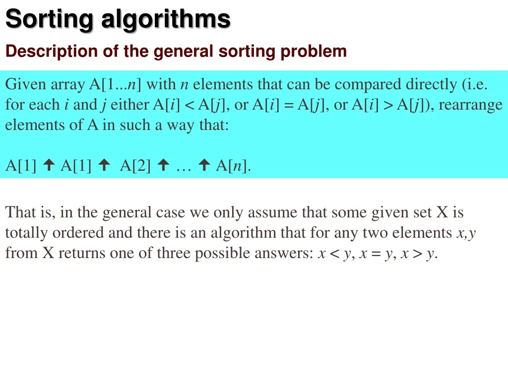
Description of the general sorting problem Given array A[1...n] with n elements that can be compared directly (i.e. for each i and j either A[i] < A[j], or A[i] = A[j], or A[i] > A[j]), rearrange elements of A in such a way that: A[1] A[1] A[2] …A[n]. That is, in the general case we only assume that some given set X is totally ordered and there is an algorithm that for any two elements x,y from X returns one of three possible answers: x < y, x = y, x > y.
To understand algorithms it is sufficient to assume that elements of array A are just integers. In practice elements of array A usually will be more complex and will have to be sorted according to some particular property (Key), e.g. (in C++) they may be defined as classes class Item { int Key; };
If elements of A are complex (use large amount of memory) it may be more efficient to construct new array B of keys, sort it, and then rearrange items in initial array according to the order of keys. Actually elements of B must contain also the information about the initial position of keys, i.e. they should be pairs (Key,Position).
Insertion Sort procedureInsertionSort(array A[1…n]): for ifrom2to n do j i x A[i] while j 1and A[j1] > x do A[j] A[j1] j j 1 A[j] x
Insertion Sort - Complexity procedureInsertionSort(array A[1...n]): for ifrom2to ndo j i x A[i] while j 1and A[j1] > x do A[j] A[j1] j j 1 A[j] x n1 0..i
Insertion Sort - Complexity Time (number of operations) – worst case: T(n) = (c1+ c2) + (c1+ 2c2) + … + (c1+ (n 1) c2) T(n) =nc1+ (1/2 n (n 1)) c2 T(n) = (n2) Space (memory) – worst case: M(n) = n +const
Insertion Sort - Complexity Average complexity? For space – obviously the same: M(n) = n +const For time – it can be shown that (n2) operations are required also in average case.
Insertion Sort - Complexity (empirical) [Adapted from M.Lamont]
Bubble Sort (version 1) procedureBubbleSort(array A[1...n]): for ifrom1to n do for jfrom2to ndo if A[j] > A[j1] then A[j] A[j1]
Bubble Sort - Complexity procedureBubbleSort(array A[1...n]): for ifrom1to n do for jfrom2to n do if A[j] > A[j1] then A[j] A[j1] n n1
Bubble Sort Complexity Worst case: T(n) = n(n–1) const = (n2) M(n) = n +const Average complexities are the same as in worst case
Bubble Sort Complexity (empirical) [Adapted from M.Lamont]
Bubble Sort (version 2) procedureBubbleSort(array A[0…n]): stop = false while stop =falsedo stop =true for jfrom2to n do if A[j] > A[j1] then stop = false A[j] A[j1]
Simple sorting algorithms - empirical complexity [Adapted from M.Lamont]
Merge Sort - Idea [Adapted from H.Lang]
Merge Sort procedureMergeSort(array A[l...r], B[l...r]): if l < rthen m l + (r l)/2 MergeSort(A[l…m], B[l…m]) MergeSort(A[m+1...r], B[m+1...r]) Merge(A[l...r], B[l...m], B[m+1...r])
Merge Sort procedure Merge(array A[l...r], B[l...m], C[m+1...r]) apos l; bpos l; cpos m+ 1 whilebpos mandcpos rdo if B[bpos] < C[cpos] then A[apos] B[bpos]; bpos bpos+ 1; apos apos+ 1 else A[apos] C[cpos]; cpos cpos+ 1; apos apos+ 1 whilebpos mdo A[apos] B[bpos]; bpos bpos+ 1; apos apos+ 1 whilecpos rdo A[apos] C[cbos]; cpos cpos+ 1; apos apos+ 1
Merge Sort - Complexity Worst case: Merge procedure: Tm(n) = n const = (n) MergeSortprocedure: T(n) = 2 T(n/2) + const + Tm(n) = 2 T(n/2) + (n) = (n log n)
Merge Sort - Complexity Worst case: MergeSortprocedure: T(n) = 2 T(n/2) + const + Tm(n) = 2 T(n/2) + (n) T(n) = (n log n) M(n) = 2 n + const(can be impoved up to 3/2 n + const) Average complexities are the same as in worst case
Quick Sort Sort - Idea [Adapted from H.Lang]
Quick Sort (not very efficient version) procedureQuickSort(array A[1...n]): if n > 1 then xA[1] (or iRandom(n);x A[i]) bpos1; cpos 1 for ifrom 1to ndo if x > A[i] then B[bpos] = A[i]; bpos bpos+ 1 if x A[i] then C[cpos] = A[i]; cpos cpos+ 1 QuickSort(B[1...bpos]); QuickSort(C[1...cpos]) Append(x,A[1...n], B[1...bpos], C[1...cpos])
Quick Sort (not very efficient version) procedure Append(x,A[1...n], B[1...bpos], C[1...cpos]) for ifrom 1 to bposdo A[i] B[i] A[bpos] = x for ifrom 1 to cposdo A[bpos+i+1] C[i]
Quick Sort - Example [Adapted from T.Niemann]
Quick Sort - Example 2 4 8 2 2 8 4
Quick Sort - Complexity Worst case: Append procedure: Ta(n) = n const = (n) QuickSortprocedure: T(n) = T(bpos) + T(cpos) + (n)+ Ta(n) = = T(bpos) + T(cpos) + (n)
Quick Sort - Complexity QuickSortprocedure: T(n) = T(bpos) + T(cpos) + (n) Case 1: bpos = cpos T(n) = 2 T(n/2) + (n) Case 2: bpos= 1, cpos = n– 1 T(n) = T(1) + T(n– 1) + (n) = (n log n) = (n2)
Quick Sort - Complexity It can be shown that the worst situation is in Case 2 (or with bpos and cpos reversed), thus QuickSort worst case time complexity is T(n) = (n2)
Quick Sort - Complexity Good news: • Average time complexity for QuickSort is (n log n) • This (inefficient) version uses 2n+ const of space, but that can be improved to n + const • On average QuickSort is practically the fastest sorting algorithm
Quick Sort - Complexity [Adapted from K.Åhlander]
Quick Sort - Complexity [Adapted from K.Åhlander]
Quick Sort - Complexity [Adapted from K.Åhlander]
Quick Sort - Complexity [Adapted from K.Åhlander]
Quick Sort - Complexity [Adapted from K.Åhlander]
Quick Sort (more efficient version) procedure QuickSort(array A[l...r]): if l < rthen i l; j r+ 1; x A[l] (or select x randomly) whilei < jdo i i+ 1 while i rand A[i] < xdo i i+ 1 j j– 1 while j l and A[j] > xdo j j– 1 A[i] A[j] A[i] A[j]; A[j] A[l] QuickSort(A[l...j–1]) QuickSort(A[j+1...r])
Quick Sort (more efficient version) i j After selecting of x move pointers i and j from start and array correspondingly and swap all pairs of elements for which A[i] > x and A[j] < x
Quick Sort (more efficient version) - example Positions: 1 2 345678910 Keys: 9111171318 41214 5 > > < after 1while: 91 5171318 4121411 > < < < after 2while: 91 5 4131817121411 < >< < after 3while: 91 513 41817121411 2 extra swaps: 41 5 9131817121411 sort sub-arrays:1 4 5 9111213141718
Shell Sort - Idea Donald Shell 1959 h1= 1 < h2< h3 < h4 < h5 < an increasing sequence of integers For given n select some hk < n. Repeatedly for inc = hk, hk-1,, h1= 1 and for sfrom 1 to inc InsertionSort the sequences A[s], A[s + inc],A[s + 2 inc], A[s + 3 inc],
Shell Sort - Idea [Adapted from H.Lang]
Shell Sort procedure ShellSort(array A[1…n]): inc InitialInc(n) whileinc 1 do for ifrominctondo j i x A[i] while j incand A[j–inc] > xdo A[j] A[j–inc] j j – inc A[j] x inc NextInc(inc,n)
Shell Sort - Example Positions: 12345678910 Keys: 9 111171318 41214 5 sort for inc = 5: 9111171318412145 9111145184121713 sort for inc = 3: 9111145184121713 4111951713121814 sort forinc= 1: 4111 9 5 17 13121814 1 4 5 91112 13141718
Shell Sort - Good increment sequences? • sequence 1, 2, 4, 8, (hi= 2i-1) is not particularly good • the “best” increment sequence is not known • sequence 1, 4, 13, 40, 121, (hi = (3i–1)/2 ) is one (of several known) that gives good results in practice
Shell Sort - Complexity • in general the finding of time complexity for a given increment sequence is very difficult • for sequence 1, 2, 4, 8, we have T(n) = (n2) • it is known that for sequence 1, 4, 13, 40, 121, T(n) = O(n1.5), but in practice it tends to perform comparably with n log n time algorithms • there exists sequences for which it has been proven that T(n) = O(n (log n)2)
Shell Sort - Complexity • it is known that for any sequence the worst case complexity T(n) = (n (log n/log logn)2) • it is not known whether average complexity T(n) = O(n log n) can be obtained
Heap Sort - procedure "Heapify" [Adapted from T.Giang]
Heap Sort - procedure "Heapify" [Adapted from T.Giang]
Heap Sort - procedure "Heapify" procedure Heapify(array A[i...j]): if RC(j) iand A[RC(j)] A[LC(j)] and A[RC(j)] < A[j] then A[j] A[RC(j)] Heapify(A[i…RC(j)]) else if LC(j) i and A[LC(j)] < A[j] then A[j] A[LC(j)] Heapify(A[i…LC(j)]) Here LC(j)= 2j–n–1 (left child) and RC(j)= 2j–n–2 (right child)