S5 H1H2: Time-Shift Approach
110 likes | 128 Vues
S5 H1H2: Time-Shift Approach. Vuk Mandic LSC Meeting MIT, 11/05/06. Time-Shift Approach. Searching for broad-band signal: 40-250 Hz For S5 H1H2 observe narrow-band structure in coherence: If it is a fluctuation of a broad-band signal, we should include it in our analysis.

S5 H1H2: Time-Shift Approach
E N D
Presentation Transcript
S5 H1H2: Time-Shift Approach Vuk Mandic LSC Meeting MIT, 11/05/06
Time-Shift Approach • Searching for broad-band signal: 40-250 Hz • For S5 H1H2 observe narrow-band structure in coherence: • If it is a fluctuation of a broad-band signal, we should include it in our analysis. • Can we check if this structure is “real”? • PEM-coherence approach (Nick) • Can identify instrumentally/environmentally correlated features. • Complete coverage? • Time-shifts • Narrow-band structure should persist over 1-sec time-scale. • Cannot distinguish instrumental lines from narrow-band GW. • Two approaches are complementary.
Detection Strategy • Cross-correlation estimator • Theoretical variance • Optimal Filter Overlap Reduction Function For template: Choose N such that:
Analysis Details • Data quality cuts significantly different from usual stochastic analysis • Using glitch triggers determined by the burst group to reject segments. • Using PSD integrals to reject additional transients. • Imposing large-σ cut to reject noisy time periods. • Reject 20% of the data. • Code-changes were necessary: • Much of the post-processing done in individual jobs. • Handling data differently (loading, filtering etc) to improve speed. • Using h(t) data up to Apr 3, 2006.
1-sec Segments • 1, 2 sec shifts • Three SNR definitions: • Gaussian Fit • Maximum over four shifts • SNR of the mean of 1-sec cases • Use maximum over the three Time-shift (sec)
0.5-sec Segments • 0.5 sec shifts • 2 Hz binning • Use SNR of the mean over the two cases.
0.25-sec Segments • 0.25 sec shifts • 4 Hz binning • Consistent with 0.5-sec and 1-sec results, but the resolution is not very good. • Will not be used in the following analysis.
Coherence Coherence
Results (1) Sensitive in the 50-230 Hz band
Results (2) • H1H2 Coherence • After cuts close to the expected exponential distribution. • Can calculate sigma for these cuts: • Sensitivity for the strong cut may get somewhat worse as we include more data and modify cut thresholds. • 10x better than H1L1 over the same data. • 5-10x better than the BBN limit.
What do we miss? • Instrumental/environmental correlations that are broad-band AND not captured by the PEM channels could be missed. • This contamination would have the same properties as the GW signal we search. • If we see such signal in H1H2 analysis, a possible approach could be to use directional H1L1 searches, which do not suffer from overlap reduction… • Possible further work: • Add more data? • Can we use the phase of Y(f)? • Improve combining different SNRs? • Optimize PEM-coherence veto parameter?