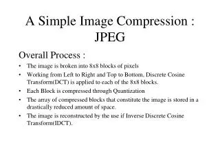
Image Compression-JPEG
Image Compression-JPEG. Speaker: Ying Wun , Huang Adviser : Jian Jiun , Ding Date 2011/10/14. Outline. Flowchart of JPEG ( Joint Photographic Experts Group ) Correlation between pixels Color space transformation-RGB to YCbCr & Downsampling KL Transform & DCT Transform

Image Compression-JPEG
E N D
Presentation Transcript
Image Compression-JPEG Speaker: Ying Wun, Huang Adviser: JianJiun, Ding Date2011/10/14
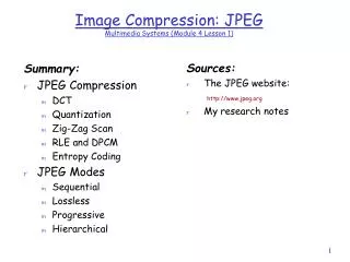
Outline Flowchart of JPEG (Joint Photographic Experts Group) Correlation between pixels Color space transformation-RGB to YCbCr & Downsampling KL Transform & DCT Transform Quantization Zigzag Scan Entropy Coding & Huffman Coding MSE & PSNR Conclusion Reference
Correlation between pixels Original Image 769KB Original Image 769KB Original Image 769KB Compressed Image 9KB Compressed Image 50KB Compressed Image 410KB • Correlation: HighLow • Compression ratio: HighLow
Color space transformation-RGB to YCbCr& Downsampling • Since luminance is more sensitive than chrominance to the human eyes, we transfer the color space from RGB to YCbCr and use downsampling(4:2:2 or 4:2:0 : downsampling; 4:4:4 : no downsampling) to reduce the information recorded in the jpeg file. • Sensitivity for human eyes: • Red(R) > Green(G) > Blue(B) • Luminance(Y) > Chromance(Cb, Cr)
Color space transformation-RGB to YCbCr& Downsampling Cb Cr Y Y Cb Cr Y Cb Cr or Y Cr Cb 4:4:4 (No downsampling) 4:2:2 (Downsampling every 2 pixels in vertical or horizontal direction.) 4:2:0(Downsampling every 2 pixels in both vertical and horizontal direction.)
KL Transform & DCT Transform • Fourier Transform & Fourier Series (1-Dimension): A signal can be expressed as a combination of sines and cosines. • KL Transform & DCT Transform (2-Dimension): A complex pattern can be expressed as a combination of many kinds of simple pattern (i.e. bases).
KLT & DCT 8x8 DCT bases • Karhunen-LoeveTransform (KLT): Every image has its own bases (i.e. different image has different bases), we need to find and save the bases information during the process of compression. • Advantage: Minimums the Mean Square Error(MSE). • Disadvantage: Computationally expensive. • Discrete Cosine Transform (DCT): Compress different image by the same bases. • Advantage: Computationally efficient. • Disadvantage: The performance of MSE is not as well as KL Transform, but it’s good enough.
KLT & DCT • Formulas of DCT: DCT Inverse-DCT Where ,
KLT & DCT Before DCT: -76, -73, -67, -62, -58, -67, -64, -55, -65, -69, -73, -38, -19, -43, -59, -56, -66, -69, -60, -15, 16, -24, -62, -55, -65, -70, -57, -6, 26, -22, -58, -59, -61, -67, -60, -24, -2, -40, -60, -58, -49, -63, -68, -58, -51, -60, -70, -53, -43, -57, -64, -69, -73, -67, -63, -45, -41, -49, -59, -60, -63, -52, -50, -34 AC terms: Small coefficient After DCT: -415.37, -30.19, -61.20, 27.24, 56.13, -20.10, -2.39, 0.46, 4.47, -21.86, -60.76, 10.25, 13.15, -7.09, -8.54, 4.88, -46.83, 7.37, 77.13, -24.56, -28.91, 9.93, 5.42, -5.65, -48.53, 12.07, 34.10, -14.76, -10.24, 6.30, 1.83, 1.95, 12.13, -6.55, -13.20, -3.95, -1.88, 1.75, -2.79, 3.14, -7.73, 2.91, 2.38, -5.94, -2.38, 0.94, 4.30, 1.85, -1.03, 0.18, 0.42, -2.42, -0.88, -3.02, 4.12, -0.66, -0.17, 0.14, -1.07, -4.19, -1.17, -0.10, 0.50, 1.68, DC terms: Large coefficient Example of DCT:
Quantization Luminance quantization table Chrominance quantization table We divide the DCT coefficients by Quantization Table to downgrade the value recorded in the jpeg file because it is hard for the human eyes to distinguish the strength of high frequency components. Quantization Table:
Quantization -415.37, -30.19, -61.20, 27.24, 56.13, -20.10, -2.39, 0.46, 4.47, -21.86, -60.76, 10.25, 13.15, -7.09, -8.54, 4.88, -46.83, 7.37, 77.13, -24.56, -28.91, 9.93, 5.42, -5.65, -48.53, 12.07, 34.10, -14.76, -10.24, 6.30, 1.83, 1.95, 12.13, -6.55, -13.20, -3.95, -1.88, 1.75, -2.79, 3.14, -7.73, 2.91, 2.38, -5.94, -2.38, 0.94, 4.30, 1.85, -1.03, 0.18, 0.42, -2.42, -0.88, -3.02, 4.12, -0.66, -0.17, 0.14, -1.07, -4.19, -1.17, -0.10, 0.50, 1.68, Quantize by lumunance quantization table -26, -3, -6, 2, 2, -1, 0, 0, 0, -2, -4, 1, 1, 0, 0, 0, -3, 1, 5, -1, -1, 0, 0, 0, -3, 1, 2, -1, 0, 0, 0, 0, 1, 0, 0, 0, 0, 0, 0, 0, 0, 0, 0, 0, 0, 0, 0, 0, 0, 0, 0, 0, 0, 0, 0, 0, 0, 0, 0, 0, 0, 0, 0, 0, We Get Many Zeros! • Example of Quantization: Before Quantization After Quantization
Low Frequency Zigzag Scan Zigzag Scan High Frequency We get a sequence after the zigzag process: −26, −3, 0, −3, −3, −6, 2, −4, 1 −4, 1, 1, 5, 1, 2, −1, 1, −1, 2, 0, 0, 0, 0, 0, −1, −1, 0, ……,0. The sequence can be expressed as: (0:-26),(0:-3),(1:-3),…,(0:2),(5:-1),(0:-1),EOB The remnants are Zeros! Run-Length Encoding
Entropy Coding & Huffman Coding DC luminance Huffman Table AC luminance Huffman Table • Key points: Encode the high/low probability symbols with short/long code length.
MSE & PSNR • Mean Square Error (MSE): f(x,y): original image f’(x,y): decoded image H: height of image W: width of image • Peak signal-to-noise ratio (PSNR): = :the maximum possible pixel value of the image
MSE & PSNR Error Image PSNR = 32.6 Correct Image PSNR = 30.4 Blind spot of MSE & PSNR: PSNR still looks fine even though we can easily find a obvious error on the right image, why? It is due to the fact that PSNR is calculated from MSE, where MSE is the “MEAN” square error.
Conclusion As a conclusion, to compress a image, first we have to reduce the correlation between pixels, then quantize the image to reduce the high frequency components, finally encode the image by entropy coding to minimize code length to get a low data rate image.
Reference [1] 酒井善則、吉田俊之 共著,白執善 編譯,影像壓縮技術 映像情報符号化,全華科技圖書股份有限公司, Oct. 2004 [2] WIKIPEDIA, “JPEG”, http://en.wikipedia.org/wiki/JPEG [3] WIKIPEDIA, “PSNR”, http://en.wikipedia.org/wiki/PSNR