Database Architecture Optimized for New Memory Access Bottleneck
Explore how memory access impacts database operations and propose solutions to address performance degradation caused by memory cache usage. Assess the efficiency of data structures and query processing algorithms to ensure optimal database performance.

Database Architecture Optimized for New Memory Access Bottleneck
E N D
Presentation Transcript
Database Architecture Optimized for the new Bottleneck: Memory Access Chau Man Hau Wong Suet Fai
Background Initial Experiment Architectural Consequences Data Structures Query Processing Algorithms Clustered Hash-Join Quantitative Assessment Conclusion Outline
The growth of hardware performance has not equally distributed CPU speed has increased roughly 70% per year Memory speed has only improved 50% at last 10 years Background Today: CPU : 3Ghz RDRAM : 800Mhz
Three aspects of memory performance Latency (physical distance limit) Bandwidth Address translate (TLB) Background Today: On die L3 Cache
To demonstrate the impact of memory access cost on the performance of database operations Simple scan test (selection on a column with zero selectivity or simple aggregation) on 4 different computers with different speed and cache size. T(s)=TCPU+TL2(s)+Tmem(s) (s is the stride size) TL2(s)=ML1(s)*lL2 ML1(s)=min(s/LSL1,1) TMem(s)=ML2(s)*lMem ML2(s)=min(s/LSL2,1) Mx—the number of cache misses LSx—the cache line sizes Lx–- the (cache) memory access latencies Initial Experiment
Initial Experiment While all machines exhibit the same pattern of performance degradation with decreasing data locality, the figure clearly show that the penalty for poor memory cache usage has dramatically increased
If no attention is paid, all advances in CPU power are neutralized due to the memory access bottleneck While memory latency stand-still, the growth of memory bandwidth does not solve the problem if data locality is low 2 proposals to address the issue, but no real solution Issuing prefetch instructions before data will be accessed Allowing the programmer to give a “cache-hint” by specifying the memory–access stride will be used Initial Experiment
In the case of sequential scan, performance is strongly determined by the record-width Vertically decomposed data structures is used to achieve better performance Storing each column in a separate binary table(BAT– an array of fixed-size two-field records, eg [OID, value]) Architectural Consequences-- Data Structures
2 space optimizations that further reduce the memory requirements in BAT Virtual-OIDs: use identical system-generated column of OIDs and compute the OID values on-the-fly Byte-encoding: use fixed-size encoding in 1- or 2-byte integer value Data Structure
Selections If selectivity is low, scan-select has optimal data locality If selectivity is high, a B-tree with a block-size equal to the cache line size is optimal Grouping and aggregation Sort/merge and hash-grouping are often used Equi-joins Hash-join is preferred. As join is the most problematic operator, let’s discuss more details.. Query Processing Algorithms
Straightforward clustering algorithm Simply scans the relation to be clustered once, insert each scanned tuple into H separate clusters, that each fit the memory cache Clustered Hash-Join • If H exceeds the number available cache lines, cache trashing occurs • If H exceeds the number of TLB entries, the number of TLB misses will explode
Splits a relation into H clusters using multiple passes Radix cluster algorithm • H=Hp (where p is passes) • B=Bp(where B is bits) • Hp=2^Bp • In the example, H1=4, H2=2, H=8, B1=2, B2=1, B=3 • When P=1, Radix cluster become straightforward cluster
The number of randomly accessed regions Hx can be kept low (smaller than the number of cache lines), while high number of H clusters can be achieved using multiple passes Allow very fine clustering without introducing overhead by large boundary structures A radix-clustered relation is in fact ordered on radix-bits. It is easy to do merge-join on the radix-bits Radix cluster algorithm
There are 3 tuning parameters for the radix-cluster algorithm The number of bits used for clustering (B), implying the number of clusters H=2^B The number of passes used during clustering (P) The number of bits used per clustering pass (Bp) Quantitative Assessment
Using 8 bytes wide tuples, consisting of uniformly distributed unique random numbers The hardware configuration is: SGI Origin2000 with one 250Mhz MIPS R10000 CPU 32Kb L1 cache (1024 lines of 32 bytes) 4Mb L2 cache (32768 lines of 128 bytes) Sufficient memory to hold all data structures 16Kb page size and 64 TLB entries Experimental Setup
When B increase to >6bits, H>64 which exceeds the number of TLB entries, the number of TLB misses increase When B >10bits, H>1024(the number of L1 cache lines, L1 misses start When B >15bits, H>32768(L2 cache lines), L2 misses start Radix Cluster Results
Only cluster sizes significantly smaller than L1 size are reasonable Isolated Join Performance • Only cluster sizes significantly smaller than L2 size are reasonable
The partitioned hash-join increase performance with increasing number of radix-bits Partitioned Hash-Join
Combined cluster and join cost for both partitioned hash-join and radix-join Radix-cluster get cheaper for less radix bits Both partitioned hash-join and radix-join get more expensive for less radix bits To determine the optimum number of B, it turns out there are 4 possible strategies Overall Join Performance
Phash L2 – partitioned hash-join on B=log2(C*12/||L2||), so the inner relation plus hash-table fits the L2 cache Phash TLB – partitioned hash-join on B=log2(C*12/||TLB||), so the inner relation plus hash-table spans at most |TLB| pages Phash L1 -- partitioned hash-join on B=log2(C*12/||L1||), so the inner relation plus hash-table fits the L1 cache Radix – radix-join on B=log2(C/8) Overall Join Performance
Overall Join Performance • Compares radix-join(thin lines) and partitioned hash-join(thick lines) over the whole bit range • Partitioned hash-join performs best with cluster size of 200 tuples • Radix with 4 tuples per cluster is better than radix 8
Overall Join Performance • Comparing radix-cluster-based strategies to non-partitioned hash-join and sort-merge-join • Cache-conscious join algorithm perform significantly better than “random-access” algorithms
Memory access cost is increasingly a bottleneck for database performance Recommend using vertical fragmentation in order to better use memory bandwidth Introduced new radix algorithms for use in join processing make optimal use of today’s hierarchical memory systems Experiment results in a broader context of database architecture Conclusion