General Relativity Physics Honours 2005

General RelativityPhysics Honours 2005 Dr Geraint F. Lewis Rm 557, A29 gfl@physics.usyd.edu.au

Black Holes (Ch 16) We are now familiar with the Schwarzschild solution in the weak-field regime (i.e. where the curvature is small and the gravitational field is weak). There is a long history (from the 1700s) that have considered strong gravitational fields, especially objects that have completely collapsed and whose gravitational fields are strong enough to prevent light from escaping i.e. a black hole. The Schwarzschild metric describes any spherical mass distribution, even a point-like distribution of mass, and hence should describe such “black holes”.

Black Holes In 1783 John Michell noted that light could not escape from a sufficiently massive and compact star, being the first to predict the existence of black holes. He argued that “corpuscles” of light would not be able to escape to infinity if their kinetic energy per unit mass (c2/2) was less than their gravitational binding energy GM/r i.e for The relativistic treatment gives the same result! In 1795, Laplace noted that “the largest bodies in the Universe may, through this cause, be invisible”.

Black Holes There is significant observational evidence for “collapsed objects” which appear to correspond to the idea of black holes. These include stellar mass black holes resulting from the collapse of massive stars, as well as super-massive black holes in Active Galaxies. GR describes these with the Schwarzschild (and other) metrics.

Schwarzschild Metric As a reminder, the Schwarzschild metric in spherical polar coordinates is; in units where G=c=1.

Singularities In the Schwarzschild metric gab/gab (with G=c=1) the metric terms depend upon ,  and terms including The metric is singular at =0 as  is undefined at this point. Such a singularity is a coordinate singularity as it can be removed by converting to cartesian coordinates. But what is happening at r=2m and r=0?

Singularities The first singularity occurs at r=2m and is known as the Schwarzschild radius or the event horizon. This is a coordinate singularity and can be removed by a coordinate transformation; as we will see later, a coordinate invariant, the Ricci scalar, is non-singular at the Schwarzschild radius. As g00=0 at r=2m, it implies the Schwarzschild sphere (at the Schwarzschild radius) is a surface of infinite redshift. However, r=0 is non-removable, even with a coordinate transformation. (Is it a “real” singularity?)

Space-Time Diagrams Consider a radial null geodesic (i.e. photons); where the differentiation is with respect to the affine parameter (or u). The Euler-Lagrange equation gives Substituting this back into the Lagrangian, it can be seen that r/ (and so is also an affine parameter).

Space-Time Diagrams The resulting equation for t vs r is Integrating this (exercise) gives Here, the first expression represents a radially outgoing null geodesic, whereas the second is a radially outgoing null geodesic.

Space-Time Diagrams • Hence, fixing  and we can draw the space-time diagram for a Schwarzschild black hole (Fig 16.7). Remembering that any future directed time-like vector (or geodesic) must sit in the light cone; • Any observer in region I (outside r=2m) takes an infinite amount of coordinate time to reach r=2m (the event horizon). • Any observer in region II (inside r=2m) cannot remain at rest and must move towards the singularity at r=0. • Aside: the Schwarzschild radius is ~6km for a neutron star, 3km for the Sun and 1cm for the Earth.

A Radially Infalling Particle The equations of motion for a radially infalling massive particle are where the dot is differentiation with respect to . We can choose k=1 which corresponds to a boundary condition at 1. If we drop a particle from a large distance with zero initial velocity;

A Radially Infalling Particle Integrating we find This is the same as the classic result! Note there is no odd behaviour as r=2m is crossed – the particle reaches the Schwarzschild radius in finite times, as well as the central singularity. Rewriting the infall in terms of coordinate time then

A Radially Infalling Particle The integral of this (which is a little messy – exercise) gives when r=2m; and with t!1 as r! 2m. Again, the particle will appear (in coordinate time) to approach the event horizon, but never cross. For a distant observer, an infalling source will appear to halt at the event horizon, fading from view as each photon (and there is a finite number of them) redshifting from view.

The Event Horizon The Schwarzschild metric presents us with some problems. While the metric represents a spherically symmetric mass distribution, clearly the singularity at r=2m appears to be problematic. As noted previously, this is a coordinate singularity which can be removed with a change of coordinate systems. This was originally seen (in 1924 and apparently ignored) by Eddington and Finkelstein (1958) who presented a new coordinate system in which the Event Horizon is not a problem.

Eddington-Finkelstein The idea is simple, make a coordinate change so that the singularity at r=2m is avoided. This is for r>2m. Now ingoing radial null geodesics are straight at 45o at -r + to (Fig 16.10). In these coordinates Clearly these coordinates are regular at r=2m and cover the entire range 0<r<1. This extends the Schwarzschild solution.

Eddington-Finkelstein Another coordinate transformation straightens out-going null geodesics. While such coordinate transformations may seem a little strange, they are no different from going from cartesian to spherical polar or cylindrical coordinates. Hence, they should be used like any other coordinate systems.

Eddington-Finkelstein The line element can be written more simply by introducing the advanced time parameter and With this, the null geodesics are given by v=constant, and gives the straight ingoing light paths (Fig 16.10).

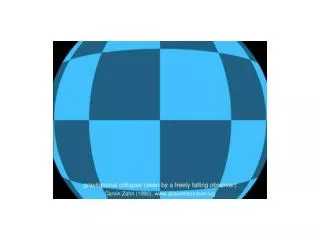
Gravitational Collapse Given the coordinate pictures we have to date, we can construct a qualitative picture for the formation of a black hole as a star collapses (Fig 16.13). As the star collapses, the density increases. There is no physical pressure that can halt the collapse and so an event horizon is formed (and all matter inside collapses to the singularity). The light cones in the vicinity of the collapse objects tip over, with those inside the event horizon tipped over by more than 45o.

Maximal Extension We have seen that changing to Eddington-Finkelstein coordinates extends the Schwarzschild solution over region I and II. Kruskal found the maximal extension (which still contains a singularity). Kruskal introduced two new coordinates t’ and x’ which are related to the radial coordinate r by This coordinate transformation straightens both ingoing and outgoing radial null geodesics.

Maximal Extension The resulting metric is The resulting space-time diagram in Kruskal coordinates is rather complicated (Fig 17.1). Light cones, however, are at 45 degrees and so the future and past are slightly easier to understand.

Maximal Extension • Regions I & II correspond to advanced Eddington-Finkelstein. • Regions I & II’ are the retarded Eddington-Finkelstein. • There is a future (black hole) singularity and a past (white hole) singularity. In Region II the future singularity is space-like and hence it is unavoidable. • Region I’ is a new feature of Kruskal space-time, an asymptotically flat space-time which is not the same as Region I.

A Graphic Illustration If this all seems a little weird, check out Andrew Hamilton’s illustrations of a change of coordinates from one to the other; http://casa.colorado.edu/~ajsh/schwp.html

Einstein-Rosen Bridge In the Kruskal coordinates, Regions I and I’ completely disconnected (the light cone in one region never overlaps with the other) except at one point. The could represent two separate universes, or two separate regions within our own universe. We can construct the evolution of an Einstein-Rosen Bridge between the two regions (at t’=0) – this is the favourite wormhole of sci-fi stories. At this point, a time-like observer could cross between one region of asymptotically flat region of space-time and another.

Maximal Compactification While we are not going to study these in detail, it is important to understand the idea. Penrose introduced a coordinate transformation that brings distant points in the Schwarzschild metric into a finite plane.

Hawking Radiation The quantum vacuum is filled with virtual particles popping in and out of existence in pairs. Hawking showed that if this occurs near the event horizon, with one particle crossing into the hole, the other can escape as a radiation. The temperature of this radiation is where rs is the Schwarzschild radius. The radiation extracts mass from the hole and rs shrinks, with T increasing catastrophically.

Charged Black Holes The addition of charge modifies the metric such that where  is the charge in the hole. This is the Reissner-Nordstrom solution. When the charge ! 0 the Schwarzschild solution is recovered. Remember that it is very unlikely that there are charged black holes in nature.

Charged Black Holes The addition of charge modifies the space-time outside of a black hole. While it is beyond this course, it is apparent that this influences the motion of neutral particles, including light! Given the metric, however, it is straight-forward to write a numerical code to look at the differing trajectories in the Schwarzschild and Reissner-Nordstrom space-times. Clearly a charged particle will respond to the “gravitational” influence of the metric as well as the EM interaction.

Singularities There are two regimes of interest. The first with 2>m2 possesses a singularity at r=0; a naked singularity. With 2<m2, then there are two coordinate singularities which occur at solutions to the equation which are

Space-Time Diagrams The influence of the two coordinate singularities is interesting, resulting in the space-time diagram shown in Figure 18.4. Crossing the outer event horizon, a particle is compelled (due to their light cone) to travel towards the centre. However, once the inner event horizon is crossed, the particle is free to avoid the singularity (but not escape it!) (You should understand Penrose compactification for this metric).

Neutral Particle Motion While we will not look at general motion of a neutral particle, it is interesting to look at some aspects of motion (Ch 18.4). Consider a radial time-like geodesic such that We can also define a (covariant) 4-velocity to be

Neutral Particle Motion This leads to the equations of motion (exercise) An analysis of these equations reveals that bound and unbound motion is possible (although the metric needs to be extended through the coordinate singularities for a complete description). Weirdly, the singularity is repulsive! But how does the particle “get out” of the hole? We need to consider the extension of the coordinates (Ch 18.5)

Neutral Particle Motion • Looking at the Penrose diagram for the charged black hole with e2<m2, the neutral particle; • Falls through outer and then inner event horizons • Falls but slows and bounces away from the singularity • Travels outwards the inner and outer horizon • However, these are now “white hole” solutions • Emerges into a different universe. • Weird!

Naked Singularities Once e2>m2 (even in the limit when m!0) the event horizons vanish. Then the hole becomes repulsive for neutral particles and even photons. The question of whether naked singularities exist in nature is hotly debated and 1969 Penrose proposed the Cosmic Censorship Hypothesis which states that naked singularities should not exist (basically because their properties are too weird). Luckily in nature no black hole should accumulate enough charge to form a naked black hole…….

A Little Spin In 1963, Kerr found the form of the metric for a mass which contains a non-zero angular momentum. This is probably the most (astro)physical of the black hole solutions. This metric is where these are Boyer-Lindquist coordinates.

A Little Spin Here, a can be thought of as an angular velocity, while am can be thought of as the angular momentum of the hole. The metric is stationary, axisymmetric and flat at large radii. Allowing a!0 we can recover the Schwarzschild metric. As with charged black holes, we will not pursue a full analysis of the Kerr metric, but will instead look at the overall properties. Note r is asymptotically the spherical polar radius and

Singularities The Kerr metric contains one intrinsic (non-coordinate) singularity which occurs at =0, so The resulting singularity is a ring with x2+y2=a2! We will not go through the detailed derivation (but read through Ch 19) but there are two pairs of additional horizons associated with the Kerr metric.

Horizons Considering g00=0 we can define two surfaces of infinite redshift Furthermore, we also have two event horizons at These are related to the inability to remain at constant radius (2nd solution) and angle (1st solution).

Horizons The resulting picture is presented in Fig 19.3 with the space-time structure similar to the Riessner-Nordstrom black hole. The result of the cross terms in the metric (d dt) is that any radially infalling particle (or light!) gains an angular velocity. The space-time is said to have been “dragged” around the hole. We will visit this again when we look at Lense-Thirring precession. At the outer surface, a particle would have to be counter-rotating at c to remain stationary. Inside this surface, the particle must rotate with the hole.

Photon Orbits Given rotation of space-time the path of light (null geodesics) in the vicinity of a Kerr black hole depend upon orientation of the encounter. This figure illustrates how the path of equatorial rays differ if they approach in a prograde or retrograde fashion.

Photon Orbits The Schwarzschild solution possesses a photon sphere in which a photon can orbit the black hole. There is a similar picture for the Kerr metric, but the orbits are more complex and requires numerical integration; http://www.physics.nus.edu.sg/~phyteoe/kerr/

Naked Again If the hole is rotating too fast (a>m) then again the event horizons merge and disappear, leaving a naked ring singularity. Unlike the charged black hole, such a “spun-up” black hole is astrophysically plausible, leading to further strong discussions about the ideas of cosmic censorship. While beyond this course, there is an analytic metric for a rotating, charged black hole, the Kerr-Newman solution.

No Hair Israel was the first to suggest that black hole collapse had to be spherical, but Wheeler extended this to say that no matter what the initial mass distribution, the memory of this shape is forgotten. The “no hair” hypothesis states that the only memory a black hole can have is their mass, angular momentum and charge. Other information can be lost through gravitational waves (although see recent arguments including Hawking).

General Relativity Physics Honours 2005