Download
1 / 26
260 likes | 427 Vues
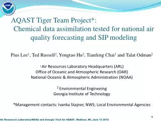
AQAST Tiger Team Project*: Chemical data assimilation tested for national air quality forecasting and SIP modeling. Pius Lee 1 , Ted Russell 2 , Yongtao Hu 2 , Tianfeng Chai 1 and Talat Odman 2 1 Air Resources Laboratory Headquarters (ARL) Office of Oceanic and Atmospheric Research (OAR)

E N D
AQAST Tiger Team Project*: Chemical data assimilation tested for national air quality forecasting and SIP modeling Pius Lee1, Ted Russell2, Yongtao Hu2, Tianfeng Chai1 and Talat Odman2 1 Air Resources Laboratory Headquarters (ARL) Office of Oceanic and Atmospheric Research (OAR) National Oceanic & Atmospheric Administration (NOAA) 2 Environmental Engineeing Georgia Institute of Technology *Management contacts: Ivanka Stajner, NWS; Local Environmental Agencies
2 Objectives: (A) To improve AQ forecasting (B) Provide IC and/or BC for SIP modeling BW SJV HOU
Moderate Resolution Imaging Spectroradiometer (MODIS) http://terra.nasa.gov/About/
Data Assimilation Methods • Optimal interpolation (OI) • Easy to apply, computationally efficient • 3D-Var • Adjusts all variables in the whole domain simultaneously. Currently, GSI is being developed at NOAA/NASA/NCAR • 4D-Var • Provides more flexibility, requires adjoint model • Kalman Filter Sandu and Chai, Atmosphere 2011
Optimal Interpolation (OI) • OI is a sequential data assimilation method. At each time step, we solve an analysis problem • We assume observations far away (beyond background error correlation length scale) have no effect in the analysis • In the current study, the data injection takes place at 1700Z daily Chai et al. JGR 2006
Objective (A): Improve PM forecast Methodology of OI: Take account for background input; Obs; and physical processes from model Observation Input OI Background Input Analysis output
Use AOD Analysis/Background as Scaling Factors CMAQ 471: 49 Adjusted species • ASO4I, ANO3I, ANH4I, AORGPAI, AECI, ACLI (6) • ASO4J, ANO3J, ANH4J, AORGPAJ, AECJ, ANAJ, ACLJ, A25J (8) • AORGAT: AXYL1J, AXYL2J, AXYL3J, ATOL1J, ATOL2J, ATOL3J, ABNZ1J, ABNZ2J, ABNZ3J, AALKJ, AOLGAJ (11) • AORGBT: AISO1J, AISO2J, AISO3J, ATRP1J, ATRP2J, ASQTJ, AOLGBJ (7) • AORGCT: AORGCJ (1) • ASO4K, ANO3K, ANH4K, ANAK, ACLK, ACORS, ASOIL (7) • NUMATKN, NUMACC, NUMCOR (3) • SRFATKN, SRFACC, SRFCOR (3) • AH2OJ, AH2OI, AH2OK (3) Tong et al. ACP 2012 for CMAQ5.0 dust module
Model & MODIS AOD on 7/4/11 Base: R=0.25 Y=0.21+0.09 X OI: R=0.34 Y=0.19+0.15 X
HMS fire detect 7/4 MODIS AOD 17 UTC 7/3 7/4/11 AOD 17 UTC 7/4 after OI OI Base Case AOD 17 UTC 7/4 MODIS AOD 17UTC 7/4 OI minus Base Case
MODIS AOD 17 UTC 7/4 7/5/11 AOD 17 UTC 7/5 after OI OI Base Case AOD 17 UTC 7/5 MODIS AOD 17UTC 7/5 OI minus Base Case
MODIS AOD 17 UTC 7/5 7/6/11 AOD 17 UTC 7/6 after OI OI Base Case AOD 17 UTC 7/6 MODIS AOD 17UTC 7/6 OI minus Base Case
MODIS AOD and AIRNow PM2.5 Correlation Chai et al. JGR 2006 http://www.star.nesdis.noaa.gov/smcd/spb/aq/
Objective (B): Provide D.A. dynamic BC for SIP modeling • WRF 3.2.1 for meteorological fields • NCEP North American Regional Reanalysis (NARR) 32-km resolution inputs • NCEP ADP surface and soundings observational data • MODIS landuse data for most recent land cover status • 3-D and surface nudging, Noah land-surface model • SMOKE 2.6 for CMAQ ready gridded emissions • NEI inventory projected to 2011 using EGAS growth and existing control strategies • BEIS3 biogenic emissions based on BELD3 database • GOES biomass burning emissions: ftp://satepsanone.nesdis.noaa.gov/EPA/GBBEP/ • CMAQ 4.6 revised to simulate gaseous & PM species • SAPRC99 mechanism, AERO4, ISORROPIA thermodynamic, Mass conservation, • Updated SOA module (Baek et. al. JGR 2011) for multi-generational oxidation of semi-volatile organic carbons
Tests with data assimilated IC/BC Simulate the period of 12Z on July 1, 2011 through 12Z on July 12, 2011 for testing assimilated PM fields as IC/BC. The tests are conducted on the 12- and 4-km grids with IC/BC modified for the 12-km grid. IC/BC of base and fdda cases are prepared using the NOAA provided data with the following 25 model species modified from the IC/BC that the original hindcast used . Model Species that replaced in IC/BC with NOAA data 25 model species ASO4J ASO4I ANH4J ANH4I ANO3J ANO3I AORGPAJ AORGPAI AECJ AECI A25J ACORS ASOIL NUMATKN NUMACC NUMCOR SRFATKN SRFACC AH2OJ AH2OI ANAJ ACLJ ANAK ACLK ASO4K
Surface O3 bias over 4 km BW domain; where fdda applied for BC Surface PM25 bias
Summary and future work • Assimilating MODIS AOD using OI method is able to improve AOD and PM2.5 predictions in selected regions. The improvement is not “yet” significant. • Dynamic BC from archived best chemical fields generated by this project can support SIP modeling. E.g. The SIP-type limited-domain modeling result over Baltimore-Washington presented was based on ingesting assimilated AOD through dynamic LBCs. • Assimilating both MODIS AOD and AIRNow PM2.5 is expected to have better results and will be tested.
On 4km SJV real-time AQ forecast for DISCOVER-AQ Jan-Feb 2013
Tentative flight routes for DISCOVER-AQ Central Valley, Jan-Feb 2013
Objective: Provide IC and/or BC for SIP modeling • 110 x 240; • Centlon= -97.00 • Centlat=40.0 • Truelat1=33.00 • Truelat2= 45.00 SJV
Surface pressure and wind barbs; Both verified reasonably well NMMB launcher run for CalNex period
Estimate Model Error Statistics w/ Hollingsworth-Lonnberg Method • At each data point, calculate differences between forecasts (B) and observations (O) • Pair up data points, and calculate the correlation coefficients between the two time series • Plot the correlation as a function of the distance between the two stations,
Horizontal Error Statistics Rz: ~ 0.9 EB2/ Eo2: ~ 9 Correlation length: ~ 160 km
Statistical metrics for high resolution AQ model evaluation -- New paradigm Stats for Daily Maximum 8-hr O3 at All AQS Sites within 4km Domain The performance measures over the 4 km resolution may not be necessarily better than over the coarser (12 km) resolution; it may be even worse if it is evaluated using the traditional evaluation metrics based on paired obs-mod data Courtesy: Daiwen Kang, CMAS 2011 Air Resources Laboratory/NOAA and Georgia Tech for AQAST, Madison, WI, June 13 2012