Download
1 / 26
260 likes | 379 Vues
Discover the fundamentals, computational methods, and applications of molecular orbital theory in organic chemistry. Learn about approximations, calculations, and the basis of this theory.

E N D
1-3- نظریه اربیتال مولکولی محاسبات اربیتال مولکولی • تيوری (بدون هیچگونه تقریب)ab initio • نیمه تجربی empirical semi • تجربی empirical
Computational Techniques: • a) Ab Initio: STO-1G, STO-3G, 3-21G, 6-31G* ,… • J. Am. Chem. Soc.; 1975, 97(6), 1319. • J. Am. Chem. Soc.; 1975, 97(6), 1338. • J. Am. Chem. Soc.; 1975, 97(6), 1347. • b) Semi Empirical: Extended Hückel, CNDO, MNDO, MNDO/3, AM1, …
MNDO:Modified Neglect of Differential Overlap J. Am. Chem. Soc.; 1977, 99(15), 4907. J. Am. Chem. Soc.; 1977, 99(15), 4899. MNDO/3: J. Am. Chem. Soc.; 1975, 97(6), 1285. J. Am. Chem. Soc.; 1975, 97(6), 1294. J. Am. Chem. Soc.; 1975, 97(6), 1302. J. Am. Chem. Soc.; 1975, 97(6), 1307. AM1: J. Am. Chem. Soc.; 1985, 107(13), 3902.
Ab Initio Calculations: a) fewer assumption b) complex calculation c) more calculation time But More Reliable Results Semi Empirical Calculations: a) using of more approximation b) less complex and faster calculation c) less calculation time Less Reliable Results
The molecular orbital theory of organic chemistryMichael J. S. Dewar. Published 1969 by McGraw-Hill in New York
Ab Initio 4-31G Calculations for CH3 Cation, Radical, and Anion Deformation from Planarity For CH3- EMin occur atb= 23.6° Fig. 1.8: Total energy as function of distortion from planarity for CH3●, CH3+, and CH3-. J. Am. Chem. Soc.; 1976, 98(21), 6483.
Properties Calculated by Molecular Orbital Theory • Geometry (bond lengths, angles, dihedrals) • Energy (enthalpy of formation, free energy) • Vibrational frequencies, UV-Vis spectra • NMR chemical shifts • IP, Electron affinity • Atomic charge distribution (...but charge is poorly defined) • Electrostatic potential • Dipole moment.
Basis of Molecular Orbital Theory • Schrödinger equation: E = H (can be solved exactly ONLY for the Hydrogen atom, but nothing larger!!)
Molecular Orbital TheoryApproximations to the MO Theory • Orbital Approximation • It is not possible to find an exact solution for the electronic wave function in a many-electron system. It can be expressed as a product of one-electron wave functions. • el(e1,e2…en)=1(e1)2(e2)…,n(en) where i are the molecular orbitals of the system. • In this expression, electron-electron interactions are neglected. More complicated expressions treat the interactions between electrons for a many-electron system.
Utilizes three approximations to allow “solution” of many-e- Schrödinger equation • Born-Oppenheimer approximation • electrons act independently of nuclei • Hartree-Fock approximation • electrons experience the ‘field’ of all other electrons as a group, not individually • LCAO • Molecular orbitals can be constructed as linear combinations of atom-centered orbitals
nucleus B R nucleus A treat R as fixed The Born-Oppenheimer approximation The nuclei (mN >> 2000 me) move relatively slow, and can be treated as stationary while the e–s move relative to them. Then solve the Schrödinger equation for the wave function of the e– alone!! This approximation is quit good for the ground state molecule. Ex) nuclei in H2 — move ~ 1 pm e– in H2 — spread ~ 1000 pm
Schrödinger equation: kinetic energy (nuc.) kinetic energy (elect.) 2 kinetic energy terms plus 3 Coulombic energy terms: (one attractive, 2 repulsive)
Schrödinger equation after Born-Oppenheimer Approximation 0 kinetic energy (nuc.) kinetic energy (elect.) 1 kinetic energy term plus 2 Coulombic energy terms: (one attractive, 1 repulsive) plus a constant for nuclei constant
نظریه اوربیتال مولکولی نظریه جدیدی است برای توجیه پیوند شیمیایی که از معادله موجی اوربیتال های اتمی ناشی می شود. از ترکیب خطی معادله موجی اوربیتال های اتمی، اوربیتال های جدیدی به دست می آیند که به آنها اوربیتالهای مولکولی می گویند. ترکیب خطی اوربیتال های اتمی Linear Combination of Atomic Orbitals “LCAO” 15
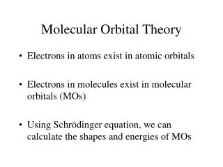
Molecular Orbital Theory There, unlike in valence bond theory, electrons are not assigned to individual bonds between atoms, but are treated as moving under the influence of the nuclei in the whole molecule. The total number of orbitals is conserved; i.e., the number of MOs equals the number of original atomic orbitals. The theory asserts that atomic orbitals no longer hold signifcant meaning after atoms form a molecule, and that electrons no longer belong to any particular atom but to the molecule as a whole.
LCAO Approximation • Electron positions in molecular orbitals can be approximated by a Linear Combination of Atomic Orbitals. • This reduces the problem of finding the best functional form for the molecular orbitals to the much simpler one of optimizing a set of coefficients (cn) in a linear equation: = c1f1 + c2f2 + c3f3 + c4f4 +… where is the molecular orbital wave function andfnrepresent atomic orbital wave functions.
1-اوربیتالهای مولکولی پیوندی 2-اوربیتالهای مولکولی ضدپیوندی ترکیب خطی اوربیتالهایpترکیب خطی اوربیتالهای s اوربیتالهای اتمی: ترکیب خطی اوربیتالهای اتمی: 18
Construction of Molecular Orbitals • 2+=(ca(1sa) + cb(1sb))2 = ca22(1sa)+cb22(1sb)+2cacb(1sa)(1sb) • ca22(1sa) is the probability of finding the electron on the 1sa atomic orbital. • 2cacb(1sa)(1sb) is the interaction term and relates to the probability of finding the electron between the atoms. • The positive term indicates bonding between the atoms.
Construction of Molecular Orbitals • 2-=(ca(1sa) - cb(1sb))2 = ca22(1sa)+cb22(1sb)-2cacb(1sa)(1sb) • ca22(1sa) is the probability of finding the electron on the 1sa atomic orbital. • In this situation, -2cacb(1sa)(1sb) is the interaction term. The electrons in this orbital are excluded from the region between the atoms. • The negative term indicates antibonding between the atoms. The surface where the electron is excluded is called a nodal surface.
LCAO-MO’s ─ 2─ bindend: anti-bindend + 2+ 7-1-2020
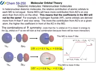
Atomic Orbital Energies and Mos 2- 2+ Here the atomic orbitals have different energies. The bonding MO is closer to atom A, the antibonding MO closer to atom B. Both atomic orbitals of same energy cA = cB
Unsymmetrical Diagram MO Energy diagram for HHe+ More Charged and also more electronegative species have lower energy levels
Methods for Construction of MO Diagrams a) Photo electron Spectroscopy (Ionization Potential; up to 20 eV, for valance electrons) b) Electron Spectroscopy for Chemical Analysis (ESCA); Binding Energy for core electrons UV or X-Ray Source Binding Energy = Photon Energy – K.E. of The Emitted Electron