Disks
This presentation covers essential concepts in storage technology, focusing on both traditional hard disk drives (HDDs) and solid-state drives (SSDs). It explores non-volatile storage, including the mechanics, properties, performance, and various interfaces of disks. Key topics include disk scheduling, data placement, RAID configurations, and the architecture of SSDs. Performance metrics such as read/write bandwidth, latency, and the impact of SSD wear-leveling techniques are also discussed. This material is essential for understanding the evolution of data storage and enhancing system performance.


Disks
E N D
Presentation Transcript
Disks Thomas Plagemann with slides from: PålHalvorsen (Ifi, UiO), Kai Li (Princeton), Tore Larsen (Ifi/UiTromsø), Maarten van Steen (VU Amsterdam)
Storage Technology [Source: http://www-03.ibm.com/ibm/history/exhibits/storage/storage_photo.html]
Contents • Non-volatile storage • Solid State Disks • Disks • - Mechanics, properties, and performance • Disk scheduling • Additional Material: • Data placement • Prefetching and buffering • Memory caching • Disk errors • Multiple disks (RAID)
Storage Properties • Volatile and non-volatile • ROM • Access (sequential, RAM) • Mechanical issues • “Wear out”
Storage Hierarchy • L1 cache • L2 cache • RAM • ROM • EPROM & flash memory (SSD) • Hard disks • (CD & DVD) • … and what about Floppy disks?
Storage Metrics • Maximum/sustained read bandwidth • Maximum/sustained write bandwidth • Read latency • Write latency
Interfaces • Parallel ATA or simply ATA • Parallel Small Computer Interface (SCSI) • Fiber Channel (FC) • Serial ATA 1.0 (SATA) • Serial ATA II (SATA II) • Serial Attached SCSI (SAS)
Interfaces [Source: http://www.intel.com/technology/serialata/pdf/np2108.pdf]
Interfaces • USB • USB 1.0/1.1: max 12 Mb/s • USB 2.0: max 480 Mb/s, sustained 10 – 30 MB/s • USB 3.0: max 4.8 Gb/s, sustained 100 – 300 MB/s • FireWire • FireWire 400: max 400 Mb/s • FireWire 800: max 800 Mb/s • eSATA: max 6 Gb/s [from: http://www.wdc.com/en/library/2579-001151.pdf]
Solid State Drives (SSD) • From the “outside” the look like hard disks • Interface • Physical formats • Inside very different to disks: • NAND Flash • Transistor arrays implemented by floating gate MOSFET • Every cell that is written to retains its charge until it is intentionally released through a “flash” of current • Erasing NAND flash needs to be done in 64, 128, or 256 KB
SSD • 2 technologies • Single Level Cell (SLC) • Multi-Level Cell (MLC) • Wear and tear • Toshiba 128GB: write capacity 80 Terabytes • Wear leveling: spread out the data • Do not defragment a SSD!! • TRIM: for delete • OSes that are not aware of SSD -> flagged as not in use • TRIM -> push delete to the SSD controller (e.g. in Windows 7)
SSD Architecture [Source: http://www.storagereview.com/ssd_architecture]
SSD vs. HDD • SSD: • Faster • Quieter • More reliable • Less power • HDD: • Cheaper
SSD Performance [Source: http://ssd.toshiba.com/benchmark-scores.html]
SSD Performance [Source: http://ssd.toshiba.com/benchmark-scores.html]
Disks • Disks ... • are used to have a persistent system • are orders of magnitude slower than main memory • are cheaper • have more capacity • Two resources of importance • storage space • I/O bandwidth • Because... • ...there is a large speed mismatch (ms vs. ns) compared to main memory (this gap will increase according to Moore’s law), • ...disk I/O is often the main performance bottleneck • ...we need to minimize the number of accesses, • ... • ...we must look closer on how to manage disks
Hard Disk Drive (HDD) Components • Electromechanical • Rotating disks • Arm assembly • Electronics • Disk controller • Cache • Interface controller
Drive Electronics • Common blocks found: • Host Interface • Buffer Controller • Disk Sequencer • ECC • Servo Control • CPU • Buffer Memory • CPU Memory • Data Channel
Mechanics of Disks Spindleof which the platters rotate around Tracksconcentric circles on asingle platter Platterscircular platters covered with magnetic material to provide nonvolatile storage of bits Disk headsread or alter the magnetism (bits) passing under it. The heads are attached to an arm enabling it to move across the platter surface Sectorssegments of the track circle separated by non-magnetic gaps.The gaps are often used to identifybeginning of a sector Cylinderscorresponding tracks on the different platters are said to form a cylinder
Disk Specifications Note 1:disk manufacturers usually denote GB as 109 whereascomputer quantities often arepowers of 2, i.e., GB is 230 • Disk technology develops “fast” • Some existing (Seagate) disksfrom 2002: Note 2:there is a difference between internal and formatted transfer rate. Internal is only between platter. Formatted is after the signals interfere with the electronics (cabling loss, interference, retransmissions, checksums, etc.) Note 3:there is usually a trade off between speed and capacity
Disk Specification SeagteCheetah 15K.6 SeagateBarracuda ES.2 Specifications from www.seagate.comon 4. 11. 2008
Disk Capacity • The size (storage space) of the disk is dependent on • the number of platters • whether the platters use one or both sides • number of tracks per surface • (average) number of sectors per track • number of bytes per sector • Example (Cheetah X15): • 4 platters using both sides: 8 surfaces • 18497 tracks per surface • 617 sectors per track (average) • 512 bytes per sector • Total capacity = 8 x 18497 x 617 x 512 4.6 x 1010 = 42.8 GB • Formatted capacity = 36.7 GB Note:there is a difference between formatted and total capacity. Some of the capacity is used for storing checksums, spare tracks, gaps, etc.
Disk Access Time • How do we retrieve data from disk? • - position head over the cylinder (track) on which the block (consisting of one or more sectors) are located • - read or write the data block as the sectors move under the head when the platters rotate • The time between the moment issuing a disk request and the time the block is resident in memory is called disk latency or disk access time
block x in memory I want block X Disk Access Time Disk platter Disk access time = Disk head Seek time +Rotational delay +Transfer time Disk arm +Other delays
Time ~ 3x - 20x x Cylinders Traveled 1 N Disk Access Time: Seek Time • Seek time is the time to position the head • - the heads require a minimum amount of time to start and stop moving the head • - some time is used for actually moving the head – roughly proportional to the number of cylinders traveled • Time to move head: number of tracks seek time constant fixed overhead “Typical” average: 10 ms 40 ms 7.4 ms (Barracuda 180) 5.7 ms (Cheetah 36) 3.6 ms (Cheetah X15)
head here block I want Disk Access Time: Rotational Delay • Time for the disk platters to rotate so the first of the required sectors are under the disk head Average delay is 1/2 revolution“Typical” average: 8.33 ms (3.600 RPM) 5.56 ms (5.400 RPM) 4.17 ms (7.200 RPM) 3.00 ms (10.000 RPM) 2.00 ms (15.000 RPM)
amount of data per tracktime per rotation Disk Access Time: Transfer Time • Time for data to be read by the disk head, i.e., time it takes the sectors of the requested block to rotate under the head • Transfer rate = • Transfer time = amount of data to read / transfer rate • Example – Barracuda 180:406 KB per track x 7.200 RPM 47.58 MB/s • Example – Cheetah X15:316 KB per track x 15.000 RPM 77.15 MB/s • Transfer time is dependent on data density and rotation speed • If we have to change track, time must also be added for moving the head Note:one might achieve these transfer rates reading continuously on disk, but time must be added for seeks, etc.
Disk Access Time: Other Delays • There are several other factors which might introduce additional delays: • CPU time to issue and process I/O • contention for controller • contention for bus • contention for memory • verifying block correctness with checksums (retransmissions) • waiting in scheduling queue • ... • Typical values: “0” (maybe except from waiting in the queue)
data size transfer time (including all) Disk Throughput • How much data can we retrieve per second? • Throughput = • Example:for each operation we have - average seek - average rotational delay - transfer time - no gaps, etc. • Cheetah X15 (max 77.15 MB/s)4 KB blocks 0.71 MB/s64 KB blocks 11.42 MB/s • Barracuda 180 (max 47.58 MB/s)4 KB blocks 0.35 MB/s64 KB blocks 5.53 MB/s
Block Size • The block size may have large effects on performance • Example:assume random block placement on disk and sequential file access • doubling block size will halve the number of disk accesses • each access take some more time to transfer the data, but the total transfer time is the same (i.e., more data per request) • halve the seek times • halve rotational delays are omitted • e.g., when increasing block size from 2 KB to 4 KB (no gaps,...) forCheetah X15typically an average of: • 3.6 ms is saved for seek time • 2 ms is saved in rotational delays • 0.026 ms is added per transfer time • increasing from 2 KB to 64 KB saves ~96,4 % when reading 64 KB } saving a total of 5.6 ms when reading 4 KB (49,8 %)
Block Size • Thus, increasing block size can increase performance by reducing seek times and rotational delays • However, a large block size is not always best • blocks spanning several tracks still introduce latencies • small data elements may occupy only a fraction of the block • Which block size to use therefore depends on data size and data reference patterns • The trend, however, is to use large block sizes as new technologies appear with increased performance – at least in high data rate systems
Disk Access Time: Complicating Issues • There are several complicating factors: • the “other delays” described earlier like consumed CPU time, resource contention, etc. • unknown data placement on modern disks • zoned disks, i.e., outer tracks are longer and therefore usually have more sectors than inner - transfer rates are higher on outer tracks • gaps between each sector • checksums are also stored with each the sectors • read for each track and used to validate the track • usually calculated using Reed-Solomon interleaved with CRC • for older drives the checksum is 16 bytes • (SCSI disks sector sizes may be changed by user!!??) inner: outer:
Writing and Modifying Blocks • A write operation is analogous to read operations • must add time for block allocation • a complication occurs if the write operation has to be verified – must wait another rotation and then read the block to see if it is the block we wanted to write • Total write time read time + time for one rotation • Cannot modify a block directly: • read block into main memory • modify the block • write new content back to disk • (verify the write operation) • Total modify time read time + time to modify + write time
Disk Controllers • To manage the different parts of the disk, we use a disk controller, which is a small processor capable of: • controlling the actuator moving the head to the desired track • selecting which platter and surface to use • knowing when right sector is under the head • transferring data between main memory and disk • New controllers acts like small computers themselves • both disk and controller now has an own buffer reducing disk access time • data on damaged disk blocks/sectors are just moved to spare room at the disk – the system above (OS) does not know this, i.e., a block may lie elsewhere than the OS thinks
Efficient Secondary Storage Usage • Must take into account the use of secondary storage • there are large access time gaps, i.e., a disk access will probably dominate the total execution time • there may be huge performance improvements if we reduce the number of disk accesses • a “slow” algorithm with few disk accesses will probably outperform a “fast” algorithm with many disk accesses • Several ways to optimize ..... • block size • disk scheduling • multiple disks • prefetching • file management / data placement • memory caching / replacement algorithms • …
Disk Scheduling • Seek time is a dominant factor of total disk I/O time • Let operating system or disk controller choose which request to serve next depending on the head’s current position and requested block’s position on disk (disk scheduling) • Note that disk scheduling CPU scheduling • a mechanical device – hard to determine (accurate) access times • disk accesses cannot be preempted – runs until it finishes • disk I/O often the main performance bottleneck • General goals • short response time • high overall throughput • fairness (equal probability for all blocks to be accessed in the same time) • Tradeoff: seek and rotational delay vs. maximum response time Is (or should) disk scheduling be preemptive or non-preemptive?
Disk Scheduling • Several traditional algorithms • First-Come-First-Serve (FCFS) • Shortest Seek Time First (SSTF) • SCAN (and variations) • Look (and variations) • …
cylinder number scheduling queue 1 5 10 15 20 25 time First–Come–First–Serve (FCFS) FCFS serves the first arriving request first: • Long seeks • “Short” average response time incoming requests (in order of arrival): 12 14 2 7 21 8 24 12 14 2 7 21 8 24
cylinder number scheduling queue 1 5 10 15 20 25 time Shortest Seek Time First (SSTF) SSTF serves closest request first: • short seek times • longer maximum response times – may even lead to starvation incoming requests (in order of arrival): 12 14 2 7 21 8 24 12 14 2 7 21 8 24
cylinder number 1 5 10 15 20 25 time SCAN SCAN (elevator) moves head edge to edge and serves requests on the way: • bi-directional • compromise between response time and seek time optimizations incoming requests (in order of arrival): 12 14 2 7 21 8 24 12 14 2 7 21 8 24 scheduling queue
cylinder number 1 5 10 15 20 25 time LOOK LOOK is a variation of SCAN: • same schedule as SCAN • does not run to the edges • stops and returns at outer- and innermost request • increased efficiency • SCAN vs. LOOK example: incoming requests (in order of arrival): 12 14 2 7 21 8 24 scheduling queue 2 7 8 24 21 14 12
Data Placement on Disk • Disk blocks can be assigned to files many ways, and several schemes are designed for • optimized latency • increased throughput • access pattern dependent
Constant angular velocity (CAV) disks equal amount of data in each track(and thus constant transfer time) constant rotation speed Zoned CAV disks zones are ranges of tracks typical few zones the different zones have different amount of data different bandwidth i.e., more better on outer tracks Disk Layout
Disk Layout • Cheetah X15.3 is a zoned CAV disk: • Always place often used data on outermost tracks (zone 0) …!? • NO, arm movement is often more important than transfer time
Data Placement on Disk • Contiguous placement stores disk blocks contiguously on disk • minimal disk arm movement reading the whole file (no intra-file seeks) • possible advantage • head must not move between read operations - no seeks or rotational delays • can approach theoretical transfer rate • often WRONG: read other files as well • real advantage • do not have to pre-determine block (read operation) size (whatever amount to read, at most track-to-track seeks are performed) • no inter-operation gain if we have unpredictable disk accesses file A file B file C
Data Placement on Disk • To avoid seek time (and possibly rotational delay), we can store data likely to be accessed together on • adjacent sectors (similar to using larger blocks) • if the track is full, use another track on the same cylinder (only use another head) • if the cylinder is full, use next (adjacent) cylinder (track-to-track seek)
file A file B file C Data Placement on Disk • Interleaved placement tries to store blocks from a file with a fixed number of other blocks in-between each block • minimal disk arm movement reading the files A, B and C(starting at the same time) • fine for predictable workloads reading multiple files • no gain if we have unpredictable disk accesses • Non-interleaved (or even random) placement can be used for highly unpredictable workloads
head block access probability block access probability cylinder number cylinder number Data Placement on Disk • Organ-pipe placement consider the usual disk head position • place most popular data where head is most often • center of the disk is closest to the head using CAV disks • but, a bit outward for zoned CAV disks (modified organ-pipe) innermost outermost disk: Note:skew dependent on tradeoff between zoned transfer time and storage capacityvs.seek time modified organ-pipe: organ-pipe:
Concluding Questions • What are the main differences between HDD and SDD? • What are the main parameter of HDD performance? • What is the goal of disk scheduling? • Would disk scheduling for SDD be useful? • Why should we not defragment SDDs?