Download
1 / 5
50 likes | 187 Vues
Control System Miniseries - Summary of Lecture 1 - 3. 06/03/2012. Core Contents of Lecture 1. Motor Output Torque. Gearbox Output Torque. Drawing a system block diagram is starting point of any control system design. Example, ball shooter of 2012 robot. Speed Error. Control Voltage.

E N D
Control System Miniseries- Summary of Lecture 1 - 3 06/03/2012
Core Contents of Lecture 1 Motor Output Torque Gearbox Output Torque • Drawing a system block diagram is starting point of any control system design. • Example, ball shooter of 2012 robot Speed Error Control Voltage Motor Voltage Wheel Speed Δω (rpm) Vctrl (volt) Vm (volt) Tm (N-m) Tgb (N-m) ωwhl (rpm) ω0 (rpm) + Control Software Jaguar Speed Controller Motor Gearbox Shooter Wheel - Controller Plant Sensor Voltage to Speed Converter Hall Effect Sensor (Voltage Pulse Generator Pulse Counter ωfbk (rpm) Vpls (volt) Pwhl (# of pulse) Measured Wheel Speed Voltage of Pulse Rate Sensor Pulse • Tip: Draw a system block diagram • On our robot, starting from shooter wheel, you can find a component connecting to another component. For example, wheel is driven by gearbox, gearbox is driven by a motor, motor is driven by speed controller, …. Physically you can see and touch most of them on our robot. • For each component, draw a block in system diagram. • Name input and output of each block, present them in symbols. Later, you will use these symbols to present mathematic relation of each block and entire system. • Define unit of each variable (symbol)
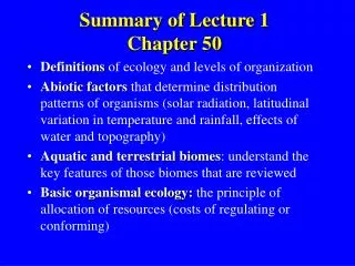
Core Contents of Lecture 2 • To a step input (the red curve in following plots), responses of system with a well designed controller should have performance as the green curves. • Green curves in both plots have optimal damping ratio (0.5 ~ 1) • But, the green curve in right figure is preferred because it has faster response (higher bandwidth) • Systems with behavior as shown in above figures can be represented by 2nd order differential equation. • Tip: We take an approach to design our control system without solving this differential equation. • Model robot system based on physics and mathematics. • Typically we will get the 2nd order differential equation as above. Then we optimize • Damping ratio: ζ = 0.5 ~ 1. • System bandwidth(close loop): ωb = 5 - 10 Hz for 50 Hz control system sampling rate
Core Contents of Lecture 3 • The characteristics of 2nd order differential equation (or a system which can be presented by the same equation) can be examined by solving special cases such as F(t) = 0 or F(t) = 1 and given initial conditions. • At this point, you can use solutions from Mr. G’s presentation for our robot control system analysis and design. Tip: use published solutions listed in table below for your simulation.
Heads-up • In rest of lectures we will get on real stuff of our robot. • First, we will model ball shooter wheel, its gearbox and motor, etc. • Second, analyze a proportional controller. • Proportion controller (P)with speed feedback is used on our shooter. • Answer why the system is always stable (thinking about damping). Can step response be faster? • Run step response test. • Answer why this system can not keep constant speed in SVR. We will introduce disturbance input in block diagram. • Third, we will change the controller to proportion – integration controller (PI) • Analyze that under which condition this system will be stable or not stable. • Program the controller on robot and see step response. • Add load to shooter and see if speed can be constant. • Fourth, we will change the controller to proportion-integration-derivative (PID) controller if we can not achieve stable operation from above design. • Modeling and analysis could be more complicated for students. But we will give a try. • We will finalize the design and tune the system for CalGames. • Then, we will get on aiming position control system design for CalGames.