Parallel Algorithm Construction
This text explores parallel algorithms for MIMD (Multiple Instruction, Multiple Data) machines, categorizing them into three main types: pipelined, partitioned, and asynchronous algorithms. Pipelined algorithms break down processes into an ordered sequence where the output of one process serves as the input to the next, enhancing efficiency through simultaneous processing. Partitioned algorithms decompose datasets into smaller chunks processed by multiple processors, while asynchronous algorithms operate independently without rigid dependencies. Each strategy offers unique advantages for optimizing computational tasks.

Parallel Algorithm Construction
E N D
Presentation Transcript
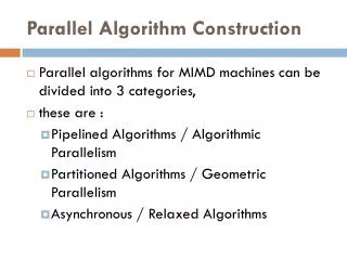
Parallel Algorithm Construction • Parallel algorithms for MIMD machines can be divided into 3 categories, • these are : • Pipelined Algorithms / Algorithmic Parallelism • Partitioned Algorithms / Geometric Parallelism • Asynchronous / Relaxed Algorithms
Pipelined Algorithms / Algorithmic Parallelism • A pipelined algorithm is an ordered set of ( possibly different ) processes in which the output of each process is the input to its successor. • The input to the first process is the input to the algorithm • The output from the last process is the output of the algorithm.
Pipelined Algorithms • Typically each processor forms part of a pipeline and • performs only a small part of the algorithm. • Data then flows through the system ( pipeline ) being operated on by each processor in succession.
Example • Say it takes 3 steps A, B & C to assemble a widget and assume each step takes one unit of time • Sequential widget assembly machine: • Spends 1 unit of time doing step A followed by 1 unit of time doing step B, followed by 1 unit of time doing step C • So a sequential widget assembler produces 1 widget in 3 time units, 2 in 6 time units etc.i.e. one widget every 3 units
Example • Pipelined widget assembly machine • Say we use a 3 segment pipeline where each of the subtasks ( A, B or C) is assigned to a segment • i.e. the machine is split into 3 smaller machines; one to do step A, one for step B and one for step C and which can operate simultaneously.
Example • The first machine performs step A on a new widget every time step and • passes the partially assembled widget to the second machine which performs step B. • This is then passed onto the third machine to perform step C
Example • This produces the first widget in 3 time units (as the sequential machine), • but after this initial startup time one widget appears every time step. • i.e. the second widget appears at time 4the third widget appears at time 5 etc.
Pipelined Algorithms • In general • if L is the number of steps to be performed • and T is the time for each step • and n is the number of items ( widgets ) • then Time Sequential = LTn • and Time Parallel = [ L + n-1 ]T
Pipelined Algorithms • T = 1, L = 100, n = 10^6 • then Tseq = 10^8 and Tpipe = 100 + 10^6 - 1 = 10^6 + 99 • Speedup = Tseq / Tpipe = 10^8 / ( 10^6 +99 ) = 100 • i.e. 100 fold increase in speed. • In general as n tends to infinity speedup tends to L.
Geometric Parallelism / Partitioned Algorithms • These algorithms arise when there is a natural way to decompose the data set into smaller "chunks" of data, • which are then allocated to individual processors. • Thus each processor contains more or less the same code but operates on a subset of the total data.
Partitioned Algorithms • The solution to these subproblems are then combined to form the complete solution. • Depending on the algorithm being solved this combining of solutions usually implies • communication synchronization among the processors. • Synchronization means constraining a particular ordering of events.
Example • if data needs to be communicated between processors after each iteration of a numerical calculation then this implies synchronization between processes. • Thus partitioned algorithms are sometimes called synchronous algorithms
Partitioned Algorithms • To illustrate the difference between pipelined and partitioned algorithms consider the following: • Say an algotithm consists of 4 parts A, B, C and D and • this algorithm is to operate on a data set E consisting of 4 subsets E1, E2 , E3 and E4 • (e.g. divide up matrix into submatrix )
Partitioned Algorithms • The pipelined algorithm would consist of 4 processors performing A, B, C, or D. • The complete data set would then pass through all 4 processors.
Partitioned Algorithms • However in the partitioned algorithm the four processors all perform A, B, C and D but only on a subset of the data
Partitioned Algorithms • i.e. In pipelined algorithms the algorithm is distributed among the processors whereas in partitioned algorithms the data is distributed among the processors.
Example • Say we want to calculate Fi = cos(sin e^sqr(xi)) for x1, x2 ,....x6 using 4 processors. • Pipelined Version
Example • F1 is produced in 4 time unitsF2 is produced at time 5i.e. time = 4 + (6-1) = 9 units==> SPEEDUP = 24 / 9 = 2.6
Example • Partitioned Version • This time each processor performs the complete algorithm i.e. cos(sin e^sqr(x)) but on its own data.
Example • i.e. time = 8 units ==> SPEEDUP = 24 / 8 = 3==> EFFICIENCY = 75% • Efficiency is calculated by dividing speedup by number of processors • E=S/n
Asynchronous / Relaxed Parallelism • In relaxed algotithms there is no explicit dependency between processes, • as occurs in synchronized algorithms. • Instead relaxed algorithms never wait for input. • If they are ready they use the most recently available data
Relaxed Parallelism • To illustrate this consider the following. • Say we have two processors A and B. A produces a sequence of numbers a1, a2 .. • B inputs ai and performs some calculation F which uses ai. • Say that B runs much faster than A.
Example • Synchronous Operation • A produces a1 passes it to B which calculates F1; • A produces a2 passes it to B which calculates F2; • i.e. B waits for A to finish ( since B is faster than A ) etc..
Example • Asynchronous Operation • A produces a1 passes it to B which calculates F1 • but now A is still in the process of computing a2 • so instead of waiting B carries on and calculates F2 ( based on old data i.e. a1 and therefore may not be the same as F2 above )and • continues to calculate F using the old data until a new input arrives • e.g. Fnew = Fold + ai
Relaxed Parallelism • The idea in using asynchronous algorithms is that all processors are kept busy and never remain idle (unlike synchronous algorithms ) so speedup is maximized. • A drawback is that they are difficult to analyse ( because we do not know what data is being used ) and • also an algorithm that is known to work ( e.g. converge) in synchronous mode may not work (e.g diverge) in asynchronous mode.
Relaxed Parallelism • Consider the Newton Raphson iteration for solving • F (x) = 0 • where F is some non-linear function • i.e. Xn+1 = Xn - F(Xn)/F'(Xn)......( 1 ) generates a sequence of approximations to the root, starting from a value X0.
Relaxed Parallelism • Say we have 3 processors • P1 : given x, P1 calculates F (x ) in time t1, units and sends it to P3 • P2 :given y, P2 calculates F'(y) in time t2 units and sends it to P3 • P3 : given a, b, c, P3 calculates d = a - b/c in time t3 units; • if | d-a | > Epsilon then d is sent to P1 and P2 otherwise d is output.
Example • Serial Mode • P1 computes F(Xn) • then P2 computes F'(Xn) • then P3 computes Xn+1 using (1) • So time per iteration is t1 + t2 + t3 • If k iterations are necessary for convergence then total time is k (t1 + t2 + t3)
Example • Synchronous Parallel Mode. • P1 and P2 compute F(Xn) and F'(Xn) simultaneously and • when BOTH have finished the values F(Xn) and F'(Xn) are used by P3 to compute Xn+1 • Time per iteration is max( t1, t2) + t3 • Again k iterations will be necessary so total time is k [ max( t1, t2) + t3]X1 = X0 - F(X0)/F'(X0) ...etc
Relaxed Parallelism • Asynchronous Parallel Mode • P1 and P2 begin computing as soon as a new input value is made available by P3 and they are ready to receive it, • P3 computes a new value using (1) as soon as EITHER P1 OR P2 provide a new input • i.e. (1) is now of the form • Xn+1 = Xn - F(SXi)/F'(Xj)