Download
1 / 46
470 likes | 784 Vues
Production and Operation Managements. Chapter 3 Aggregate Planning. Professor JIANG Zhibin Department of Industrial Engineering & Management Shanghai Jiao Tong University. Contents Introduction Aggregate Units of Production; Costs in Aggregate Planning; A Prototype Problem;

E N D
Production and Operation Managements Chapter 3 Aggregate Planning Professor JIANG Zhibin Department of Industrial Engineering & Management Shanghai Jiao Tong University
Contents • Introduction • Aggregate Units of Production; • Costs in Aggregate Planning; • A Prototype Problem; • Solution of Aggregate Planning Problem by LP; Chapter 3 Aggregate Planning
Aggregate planning, also called macro planning, decides how many employees the firm should retain and, for a manufacturing firm, the quantity and the mix of products to be produced. • Assumption: demand is deterministic, or known in advance. Introduction(1)
New one in dynamic environment: manufacturing is outsourced (Supply Chain) • Sun Microsystems is a successful example; • Focus on product innovation and design rather than manufacturing; Introduction(1)
Aggregate planning involves several basic competing objectives. • Make frequent and large changes in size of labor force: a chase strategy to react quickly to anticipated changes in demand, cost effective, but a poor long-term strategy; • Retain a stable workforce: results in larger buildups of inventory during period of low demand ; • Develop a production plan for a firm to maximize profit over the planning horizon subject to constraints on capacity. • AP methodology is designed to translate demand forecast into blueprint for planning staffing and production level for a firm over a predetermined planning horizon; Introduction(2)
Describe aggregate units in the following situations: • In terms of “average’ item-when the items produced are similar, e.g. cars, computers; • In terms of weights (tons of steel), volume (gallons of gasoline), amount of work required (worker-years of programming time), and dollar value (value of inventory in dollars)-when many kinds of items are produced; • Appropriate aggregating schema are determined by context of the particular planning problem and the level of the aggregation to be required. Aggregate Units of Production
Example 3.1: Decide on aggregating schema for the manager of a plant that produces six models of washing machines to determine the workforce and production levels. Aggregate Units of Production
One possibility is to define aggregate unit as one dollar of output • Unfortunately, it is impossible since the selling prices of the various models are not consistent with the number of worker-hours required to produce them. • Given amount of dollars of output, we could not know the total WH required. Aggregate Units of Production 4.2/285=0.0147WH/$ 5.4/525=0.008WH/$
Fact: the percentages of the total number of sales for these six models have been fairly constant (32% ,21%, 17%, 14%, 10% and 6% for six models respectively) • Define the aggregate unit of production as a fictitious washing machine requiring .324.2+.21 4.9+.17 5.1+.14 5.2+.10 5.4+.06 5.8=4.856 hrs of labor time. • Problem: Given number of washing machines to be produced, say 10,000, could we know the total WH required? Aggregate Units of Production
Defining an aggregate unit of production at higher level of the firm is more difficult; • When the firm produces a large of products, a natural aggregate unit is sales dollars; • Aggregate planning is closely related to hierarchical production planning (HPP). HPP considers workforce sizes and production rates at different levels of the firm. The recommended hierarchy is as follows: • Items-correspond to individual models of washing machines; • Families-a group of items, e.g. all washing machines; • Types-groups of families, e.g. large house appliances; Aggregate Units of Production
Fig 3-2 Cost of Changing the Size of the Workforce (1) Smoothing cost: Occurs as result of changing the production level from one period to the next. • Cost for changing size of workforce-advertise positions; interview prospective employees, and training new hires; • Assumed to be linear; Costs in Aggregate Planning
$ Cost Slope = Ci Slope = CP Negative--Back-orders Positive--Inventory • Fig.3-3 Holding and Back-Order Costs (2) Holding costs: Occurs as a result of having capital tied up in inventory. • Always assumed to be linear in the number of units being held at a particular point in time; • For aggregate planning, it is expressed in terms of dollars per unit held per planning period; (e.g. 100 $/month for one item) • Charged against the inventory remaining on hand at the end of the planning period; Aggregate Units of Production • At the beginning: 50 • Week 1: In 100 • Week 2: Out 130 • Week 3 In 30 • Week 4 Out 30 • Charge only 20
$ Cost Slope = Ci Slope = CP Negative--Back-orders Positive--Inventory • Fig.3-3 Holding and Back-Order Costs Aggregate Units of Production (3) Shortage costs- • Shortage occurs when demands are higher than anticipated; • For aggregate planning, it is assumed that excess demand is backlogged and filled in a future period; • In a highly competitive situation, the excess demand may be lost---lost sales; • Generally considered to be linear.
(4) Regular time costs: Involve the cost of producing one unit of output during regular working hours; • Actual payroll cost of regular employees working on regular time; • Direct and indirect costs of materials; • Other manufacturing expense; Aggregate Units of Production (5) Overtime and subcontracting costs: Costs of production units not produced on regular time; • Overtime-production by regular-time employees beyond work day; • Subtracting-the production of items by an outside supplier; • Assumed to be linear; (6) Idle time costs: Underutilization of workforce; • In most contexts, the idle time cost is zero; • Idle time may have other consequences for the firm, e.g. if the aggregate units are input to another process, idle time on the line could result in higher costs to subsequent processes.
Example 3.2 Densepack is to plan workforce and production level for six-month period Jan. to June. The firm produces a line of disk drives for mainframe computers. Forecast demand over the next six months for a particular line of drives in a plant are 1,280, 640, 900, 1,200, 2,000 and 1,400. There are currently (end of Dec.) 300 workers employed in the plant. Ending inventory in Dec. is expected to be 500 units, and the firm would like to have 600 units on hand at the end of June. A Prototype Problem
How to incorporate the starting and ending inventory constraints into formulation?-the simplest way is to modify the values of the predicated demand; • Define : the net predicated demand in period 1 =(the predicated demand) – (initial inventory); • If there is ending inventory constraint, this amount should be added to the demand in period T; A Prototype Problem
How to handle minimum buffer inventories required? -By modifying the predicted demand. • If there is a minimum buffer inventory required in every period, this amount should be added only to the first period’s demand; A Prototype Problem Problem: Why should we require the minimum buffer inventory?
How to handle minimum buffer inventories? -By modifying the predicted demand. (Cont.) • If there is a minimum buffer inventory required in only one period, this amount should be added to that period’s demand, and subtracted from the next period’s demand; A Prototype Problem
Fig. 3-4 A Feasible Aggregate Plan for Densepack If the shortage is not permitted, the cumulative production must be at least as great as cumulative net demand each period-Feasible AP A Prototype Problem AP: Any curve above the accumulated net demand
How to make cost trade-offs of various production plans? Only consider three costs: • CH=Cost of hiring one worker=$500; • CF=Cost of firing one worker=$1,000; • CI=Cost of holding one unit of inventory for one month=$80 A Prototype Problem
Translate aggregate production in units to workforce levels: • Use a day as an indivisible unit of measure (since not all month have equal number of working days) and define: • K=Number of aggregate units produced by one worker in one day. • A known fact: over 22 working days, with the workforce constant at 76 workers, the firm produced 245 disk drives. • Average production rate=245/22=11.1364 disk drives per day; • One worker produced an average of 11.1364/76=0.14653 drive in one day. K=0.14653. A Prototype Problem
Two alternative plans for managing workforce: • Plan 1 is to change workforce each month in order to produce enough units to most closely match the demand pattern-zero inventory plan; • Plan 2 is to maintain the minimum constant workforce necessary to satisfy the net demand-constant workforce plan; A Prototype Problem
P1: Zero Inventory Plan (Chase Strategy) –minimize inv. level. A Prototype Problem Table 3-1 Initial Calculation for Zero Inv. Plan for Denspack
The number of workers employed at the end of Dec. is 300; • Hiring and firing workers each month to match forecast demand. Table 3-2 Zero Inv. Aggregate Plan for Densepack A Prototype Problem
The total cost of this production plan is obtained by multiplying the totals at the bottom of Table 3-2 by corresponding unit cost: • 755500+145 1000+30 80=$524,900; • In addition, the cost of holding for the ending inventory of 600 units, which was considered as the demand for June, should be included in holding cost: 600 80=$48,000 • The total cost= $524,900+$48,000=$572,900. • Note: the initial inventory of 500 units does not enter into the calculation because it will be netted out during the month January. A Prototype Problem
It is possible to achieve zero inventory at the end of each planning period ? No! Since it is impossible to have a fractional number of workers. • It is possible that ending inventory in one or more period could build up to a point where the size of the workforce may be reduced by one or more workers. A Prototype Problem
P2 Evaluation of the Constant Workforce Plan-to eliminate completely the need for hiring and firing during the planning horizon. • In order not incur the shortage in any period, compute the minimum workforce required for every month in the planning horizon. • For January, the net cumulative demand is 780 and units produced per worker is 2.931, thus the minimum workforce is 267(780/2.931) in Jan; • Units produced per worker in Jan. and Feb. combined=2.931+3.517=6.448, and the cumulative demand is 1,420, then the minimum workforce is 221(1420/6.448) to cover both Jan. and Feb. • Go on computing in the same way. A Prototype Problem
Table 3-3 Computation of the Minimum Workforce Required by Denspack A Prototype Problem The minimum number of workers required for entire six-month planning horizon is 411, requiring hiring 111 new workers at the beginning of Jan.
Table 3-4 Inventory Level for Constant Workforce Schedule A Prototype Problem • The total cost is (5,962+600)80+111 500=580,460>569,540 for P1; • P2 is preferred because it has no large difference from P1 in cost, but keeps workforce stable.
Fig. 3-4 A Feasible Aggregate Plan Mixed Strategy and Additional Constraints • The zero inventory plan and the constant workforce strategies are to target one objective; • Combining the two plans may results in dramatically lower costs; • Figure 3-4 shows the constant workforce strategy (a straight line-a fixed production rate). A Prototype Problem the constant workforce strategy The zero inventory plan
Fig. 3-4 A Feasible Aggregate Plan Mixed Strategy and Additional Constraints Suppose that we may use two production rates (2 straight lines): • Make net inventory at the end of April to be zero (P1) by producing enough in each of the four months Jan. through April to meet the cumulative net demand each month: produce 3,520/4=880 units in each of the first four months; • The May and June production is then set to 2,000, exactly matching the net demand in these months. A Prototype Problem The two lines are above the cumulative net demand, the plan is feasible
Fig. 3-4 A Feasible Aggregate Plan A Prototype Problem
Fig. 3-4 A Feasible Aggregate Plan The graphical solution for additional constraints. a constraint on the slope of the straight line. • Capacity limitation: the production capacity of the plan is only 1,800 units per month • One feasible solution: produce 980 in each of the first four months and 1,800 in each of the last two months. (Slopes of the two segmental lines 1800) A Prototype Problem Just approach the cap. limit Lower than the cap. limit
Linear Programming (LP) is used to determine values of n nonnegative variables to maximize or minimize a linear function of these variables that is m linear constraints of these variables. Aggregate Planning by Linear Programming Cost Parameters CH=Cost of hiring one worker; CF= Cost of firing one worker; CI= Cost of holding one unit of stock for one period; CR= Cost of producing one unit product on regular time; CO= Incremental cost of one unit on overtime; CU= Idle cost per unit of production; CS= Cost of subcontract one unit of production; nt=Number production days in period t; K=Number of aggregate units produced by one worker in one day; I0=Initial inventory on hand at the start of the planning horizon; W0=Initial workforce at the start of the planning horizon; Dt=Forecast of demand in period t;
Problem Variables: • Wt=Workforce level in period t; • Pt=Production level in period t; • It=Inventory level in period t; • Ht=Number of workers hired in period t; • Ft=Number of workers fired in period t; • Ot=Overtime production in units; • Ut=Worker idle time in units (underutilized time); • St=Number of units subcontracted from outside; Aggregate Planning by Linear Programming • If Pt> KntWt : the number of units produced on overtime : Ot=Pt-KntWt; • If Pt< KntWt : the idle time is measured in units of production rather than in time, Ut= KntWt - Pt;
Constraints-Three sets of constraints to ensure conservation of labor and that of units • Conservation of workforce constraints • Wt=Wt-1+Ht-Ft; for 1t T Aggregate Planning by Linear Programming 2. Conservation of units constraints It=It-1+Pt+St-Dt; for 1t T 3T constraints 3. Conservation of relating production level to workforce levels Pt=Knt Wt+Ot-Ut; for 1t T • 4. Others • Non negative constraints; • Given I 0, IT, and W0.
Objective function-tochoose variables Wt, Pt, It, Ht, Ft,Ot, Ut and St (total 8T) to Aggregate Planning by Linear Programming • Subject to • the above 3T constraints, • nonnegative constraint: Wt, Pt, It, Ht, Ft,Ot, Ut and St0, and • I0, IT, and W0.
Rounding the Variables • Some variables such as It, Wt, Ft, Ht should be integers; • May calculate by integer linear programming, however, may be too complex; • Results of LP should be rounded up- by Conservative approach • Round Wt to the next larger integer, and then calculate Ht, Ft, and Pt; • Always feasible solution, but rarely optimized; Aggregate Planning by Linear Programming • Additional constraints • OtUt=0-either one is zero in case that there are both overtime an idle production in the same period ; • HtFt=0- either in case of hiring and firing workers in the same period • Both the two constraints are linear;
Extensions • Account for uncertainty in demand by minimum buffer inventory Bt: ItBt, for 1tT, where Bt should be specified in advance; • Capacity constraints on amount of production: PtCt; • In some cases, it may be desirable to allow demand exceed the capacity. To treat the backlogging of excess demand, the inventory needs to be expressed in terms of two different non-negative variables It+ and It-, such that It= It+ - It-, and holding cost is charged against It+, while the penalty cost for back orders against It-. • Convex piece-linear functions-composed of straight-lines segments; Figure 3-5 Aggregate Planning by Linear Programming
Fig. 3-5 A Convex Piecewise-Linear Function Aggregate Planning by Linear Programming Cost of hiring workers, the marginal cost of hiring one additional worker increases with number of workers that have been already hired.
Since no subcontracting, overtime, or idle time allowed, and the cost coefficients are constant with respect to time, the objective function is simplified as Solving AP Problems by LP: An Example (3.2) W1-W0-H1+F1=0; W2-W1-H2+F2=0; W3-W2-H3+F3=0; W4-W3-H4+F4=0; W5-W4-H5+F5=0; W6-W5-H6+F6=0; P1-I1+I0=1,280; P2-I2+I1=640; P3-I3+I2=900; P4-I4+I3=1,200; P5-I5+I3=2,000; P6-I6+I5=1,400; P1-2.931W1=0; P2-3.517W2= 0; P3-2.638W3=0; P4-3.810W4=0; P5-3.224W5=0; P6-2.198W6=0; Wi, Pi, Ii, Fi, Hi (i=1-6) 0; W0=300, I0=500, I6=600
Solved by LNGO system; • The value of objective function is $379,320.90, considerably less than that obtained by either P1 and P2, since this value is obtained by fractional values of variables . • Rounded up result: the total cost=465 500+1,00027+900 80=$379,500 Solving AP Problems by LP: An Example (3.2)
In-class quiz: 1) What is a feasible aggregate plan? 2) What does aggregate plan under chaise strategy look like, and how about that under constant workforce?
Homework for Chapter 3 • P140 Q14 • P141 Q15,16