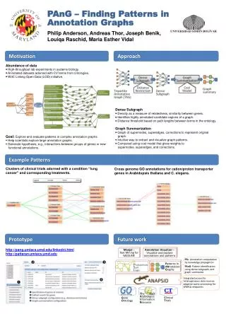
Finding Cross Genome Patterns in Annotation Graphs
This research focuses on identifying cross-genome patterns in annotation graphs, particularly within gene families. By leveraging well-curated datasets such as TAIR, WormBase, and FlyBase, the study employs methods to analyze the relationships between genes and their annotations derived from controlled vocabularies like Gene Ontology (GO) and Plant Ontology (PO). The analysis involves case studies that validate cross-genome gene functionalities, utilizing metrics for distance and similarity in annotations. The project aims to uncover interesting patterns that could lead to new biological discoveries.

Finding Cross Genome Patterns in Annotation Graphs
E N D
Presentation Transcript
Finding Cross Genome Patterns in Annotation Graphs Joseph Benik, Caren Chang, Louiqa Raschid University of Maryland Maria-Esther Vidal, Guillermo Palma Universidad Simon Bolvar Andreas Thor University of Leipzig Thanks to Heven Sze and Eic Haag NSF grants IIS0960963 and DBI1147114
Finding Cross Genome Patterns Across Gene Families in Annotation Graphs
Agenda • Motivation • Overview of PAnG (Patterns in Annotation Graphs) and PattArAn (patterns in Arabidopsis annotation) • DSG and GS • Distance metrics and similarity metrics • Annotation similarity • Case Study for Cross Genome Validation • Case Study Across Gene Families
Motivation • Many well curated model organism datasets such as TAIR, WormBase, FlyBase, etc. • Biological concepts, e.g., genes or proteins (or drugs and diseases and clinical trials) are annotated with controlled vocabulary terms from ontologies such as GO, MeSH, SNOMED, NCI Thesaurus. • We focus on genes, GO annotations and PO annotations. • Annotation evidence – nodes and edges to controlled vocabulary (CV) terms form a graph that captures meaningful knowledge. • Sense making of annotation graphs can explain phenomena, identify anomalies and potentially lead to discovery.
Genes are annotated with Gene Ontology (GO) and Plant Ontology (PO) terms • Dataset = set of genes and associated triplets. • Triplet (gene, GO, PO) • Pattern is a set of triplets (across genes, families, genome) • Link prediction (gene, GO) – a new functional annotations for a gene. • Patterns (set of tiplets) can represent a complex biological phenomenon.
PAnG Workflow • Dense Subgraph (optional) • Identify interesting regions, i.e., highly connected subgraphs • Graph summarization: • Identify basic pattern (structure) of the graph
Dense Subgraph • Motivation: graph area that is rich or dense with annotation is an “interesting region” • Density of a subgraph = number of induced edges / number of vertices • Tripartite graph with node set (A, B, C) is converted into bipartite graph with (A, C) • Weighted edges = number of shared b’s • Apply technique of [1] • Distance restriction for DSG possible • Hierarchically (poly) arranged ontology terms • All node pairs (A,A) and nodes pairs (C,C) are within a given distance [1] Saha et al. Dense subgraphs with restrictions and applications to gene annotation graphs. RECOMB, 2010
Graph Summarization • Minimum description length approach [2] • Loss-free; employs cost model • Graph summary = Signature + Corrections • Signature: graph pattern / structure • Super nodes = complete partitioning of nodes • Super edges = edges between super nodes = all edges between nodes of super nodes • Corrections: edges e between individual nodes • Additions: e G but e signature • Deletions: e G but e signature HY5 PO_9006 PHOT1 PO_20030 CIB5 CRY2 PO_37 COP1 PO_20038 CRY1 = HY5 PO_9006 PHOT1 PO_20030 CIB5 CRY2 PO_37 COP1 PO_20038 CRY1 [2] Navlakha et.al. Graph summarization with bounded error. SIGMOD, 2008
Cross Genome Case Study • Dataset At_8 and Ce_9 • 8 Arabidopsis genes in families labeled NHX or SOS • 9 C. elegans genes in families labeled nhx or pbo • Dataset At_37 and Ce_53 • 37 Arabidopsis genes • 53 C. elegans genes annotated ion transport and/or divalent cations.
Cross Family Case Study • 10 families of Arabidopsis transporter genes; 20 genes from each family. • 3 families of C. elegans genes: • slowly evolving actins and histones. • dynamically evolving heat shock proteins (HSP).
Distance/Similarity metrics • Normalized distance [0.0, 1.0] • Similarity = (1 – distance); Similarity = 1.0 (identical) • Taxonomic similarity/lexical similarity/IR based similarity • Why do we need similarity of (GO,GO) and/or (PO,PO) terms in a pattern? • Can we use path length as distance? • *real* distance.
(8,16) is more similar than (11,12) (1-0.09) > (1-0.5) .91 > 0.5 dtax (1-0.17) > (1.0.66) .83 > 0.44 dps
Distance distribution for path length 1 and 2 • For 1 • For 2
Annotation similarity Given 2 genes and their sets of GO annotations A1 and A2 we define annotation similarity as follows:
Cross Genome Validation: At_8 Deletion: NHX6 not annotated with sodium ion transmembrane transporter
Cross Genome Validation: Ce_9 Outlier
Questions? PAnG/PSL/ANAPSID/Manjal