Law of Supply

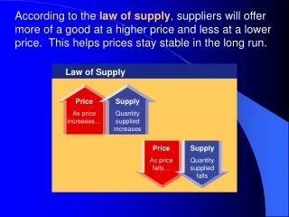
1. Law of Supply Price As price increases… Supply Quantity supplied increases Price As price falls… Supply Quantity supplied falls According to the law of supply, suppliers will offer more of a good at a higher price and less at a lower price. This helps prices stay stable in the long run.

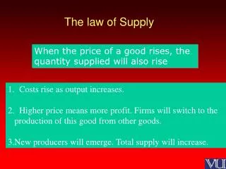
2. How Does the Law of Supply Work? • Economists use the term quantity supplied to describe how much of a good is offered for sale at a specific price. • The promise of increased revenues when prices are high encourages firms to produce more. • EX: Beluga Caviar $120/oz. • New “Kentucky Spoonfish” caviar- $10/oz. • Rising prices draw new firms into a market and add to the quantity supplied of a good. • Firms or sellers are “price takers” • When supply looks like it’s fixed—PRICES RISE

3. An example of Supply • The 1970s energy crisis encouraged countries to look to nuclear power. • Public utility companies stockpiled Uranium. • Uranium prices rose. • Entrepreneur-explorers discovered new deposits in Australia, Africa, and North America that were worth mining at the higher prices. • Slow expansion of nuclear power, combined with bulging stockpiles brought the pirce back down—to 1/8 of their highest price.

4. Market Supply Schedule Price per slice of pizza Slices supplied perday $.50 1,000 $1.00 1,500 $1.50 2,000 $2.00 2,500 $2.50 3,000 $3.00 3,500 • A market supply scheduleis a chart that lists how much of a good all suppliers will offer at different prices.

5. Market Supply Curve 3.00 2.50 2.00 1.50 1.00 .50 0 Supply Price (in dollars) 0 500 1000 1500 2000 2500 3000 3500 Output (slices per day) • A market supply curve is a graph of the quantity supplied of a good by all suppliers at different prices. Chapter 5, Section 1

6. Supply A shift of the supply curve due to a change in ceteris paribus conditions. Quantity Supplied Movements along the supply curve due to changes in the price of a good. Comparing Terminology

7. What are the ceteris paribus Assumptions that affect “Supply?” • Input Prices (if the price of batteries increases, car manufacturers will make fewer cars—they can’t afford to make more) • Technology (Bessemer process for making steel made it much cheaper to produce) • Taxes or the level of subsidies • Expectations • Government regulations (cigarette production) • “Z-factor”: Weather for crops, etc.

8. Elasticity of Supply • Elasticity of supply is a measure of the way quantity supplied reacts to a change in price • An elastic supply is very sensitive to changes in price • If supply is not responsive to changes in price, demand is considered inelastic. • Elasticity is affected by TIME. In the short run, a firm cannot easily change its output level, so supply is inelastic. In the long run, firms are more flexible, so supply can become more elastic. • Elasticity of Supply= (∆ % Quantity Supplied) / (∆% Price)

9. Section 1 Review 1. What is the law of supply? • (a) The lower the price, the larger the quantity supplied. • (b) The higher the price, the larger the quantity supplied. • (c) The higher the price, the smaller the quantity supplied. • (d) The lower the price, the more manufacturers will produce the good. 2. What happens when the price of a good with an elastic supply goes down? • (a) Existing producers will expand and some new producers will enter the market. • (b) Some producers will produce less and others will drop out of the market. • (c) Existing firms will continue their usual output but will earn less. • (d) New firms will enter the market as older ones drop out.

10. Production worksheet

11. Marginal Product of Labor Labor (number of workers) Output (beanbags per hour) Marginal product of labor 0 0 — 1 4 4 2 10 6 3 17 7 4 23 6 5 28 5 6 31 3 7 32 1 8 31 –1 A Firm’s Labor Decisions • Business owners have to consider how the number of workers they hire will affect their total production. • The marginal product of labor is the change in output from hiring one additional unit of labor, or worker.

12. Stages of Production • Stage I (increasing returns): Marginal output increases with each new worker. Companies are tempted to hire more workers. • Stage II (diminishing returns): total production keeps growing with each new worker, but the rate of increase is smaller • Stage III (negative returns): Marginal product become negative, decreasing total plant output. Yes, this can really happen.

13. Increasing, Diminishing, and Negative Marginal Returns Increasing marginal returns 8 7 6 5 4 3 2 1 0 –1 –2 –3 Diminishing marginal returns • Diminishing marginal returns occur when marginal production levels decrease with new investment. Negative marginal returns Marginal Product of labor (beanbags per hour) 1 2 3 4 5 6 7 8 9 • Negative marginal returns occur when the marginal product of labor becomes negative. Labor(number of workers) Marginal Returns • Increasing marginal returns occur when marginal production levels increase with new investment.

14. Production Costs • A fixed cost is a cost that does not change, regardless of how much of a good is produced. Examples: rent and salaries • Variable costs are costs that rise or fall depending on how much is produced. Examples: costs of raw materials, some labor costs. • The total costequals fixed costs plus variable costs. • The marginal cost is the cost of producing one more unit of a good. • EX: A self-service gas station has high fixed costs but low variable costs.

15. Production Costs Beanbags (per hour) Fixed cost Variable cost Total cost (fixed cost + variable cost) Marginal cost Marginal revenue (market price) Total revenue Profit(total revenue – total cost) 0 1 2 3 4 $36 36 36 36 36 $0 8 12 15 20 $36 44 48 51 56 — $8 4 3 5 $24 24 24 24 24 $0 24 48 72 96 $ –36 –20 0 21 40 5 6 7 8 36 36 36 36 27 36 48 63 63 72 84 99 7 9 12 15 24 24 24 24 120 144 168 192 57 72 84 93 9 10 11 12 36 36 36 36 82 106 136 173 118 142 172 209 19 24 30 37 24 24 24 24 216 240 264 288 98 98 92 79 • Total revenue is the number of units sold multiplied by the average price per unit. • Marginal revenue is the additional income from selling one more unit of a good. It is usually equal to price. To determine the best level of output, firms determine the output level at which marginal revenue is equal to marginal cost.

16. Section 2 Review 1. What are diminishing marginal returns of labor? • (a) Some workers increase output but others have the opposite effect. • (b) Additional workers increase total output but at a decreasing rate. • (c) Only a few workers will have to wait their turn to be productive. • (d) Additional workers will be more productive. 2. How does a firm set his or her total output to maximize profit? • (a) Set production so that total revenue plus costs is greatest. • (b) Set production at the point where marginal revenue is smallest. • (c) Determine the largest gap between total revenue and total cost. • (d) Determine where marginal revenue and profit are the same.

17. Input Costs and Supply • Any change in the cost of an input such as the raw materials, machinery, or labor used to produce a good, will affect supply. • As input costs increase, the firm’s marginal costs also increase, decreasing profitability and supply. • Input costs can also decrease. New technology can greatly decrease costs and increase supply.

18. Gov’t Influences on Supply By raising or lowering the cost of producing goods, the government can encourage or discourage an entrepreneur or industry. • A subsidy is a government payment that supports a business or market. Subsidies cause the supply of a good to increase. • The government can reduce the supply of some goods by placing an excise tax on them. An excise tax is a tax on the production or sale of a good. • Regulation occurs when the government steps into a market to affect the price, quantity, or quality of a good. Regulation usually raises costs.

19. Other Factors Influencing Supply The Global Economy • The supply of imported goods and services has an impact on the supply of the same goods and services here. Government import restrictions will cause a decrease in the supply of restricted goods. Future Expectations of Prices • Expectations of higher prices will reduce supply now and increase supply later. Expectations of lower prices will have the opposite effect. Number of Suppliers • If more firms enter a market, the market supply of the good will rise. If firms leave the market, supply will decrease.

20. Section 3 Review 1. What affect does a rise in the cost of raw materials have on the cost of a good? • (a) A rise in the cost of raw materials lowers the overall cost of production. • (b) The good becomes cheaper to produce. • (c) The good becomes more expensive to produce. • (d) This does not have any affect on the eventual price of a good. 2. When government actions cause the supply of a good to increase, what happens to the supply curve for that good? • (a) It shifts to the left. • (b) It shifts to the right. • (c) It reverses direction. • (d) The supply curve is unaffected.

21. Long and Short Run Aggregate Supply • Many economists believe that costs ultimately move with the price level, and that as a result, in the long run the AS curve is vertical • Initially the economy is in equilibrium at a price level of P0 and an aggregate output of Y0 (the point at which AD0 and AS0 intersect). Now imagine a shift in AD from AD0 to AD1. In response to the shift both, the price level and aggregate output rise in the short run, to P1 and Y1. Now suppose costs fully adjust to price in the long run. AS will shift left, from AS0 to AS1, and in the final analysis, if costs and prices have increased by the same percentage, then aggregate output will be back at Y0. Connecting the two long-run equilibrium points in the figure above yields the long-run aggregate supply curve, labeled LRAS in the figure above.