Data Mining Techniques Outline

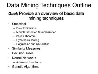
1. Data Mining Techniques Outline Goal:Provide an overview of basic data mining techniques • Statistical • Point Estimation • Models Based on Summarization • Bayes Theorem • Hypothesis Testing • Regression and Correlation • Similarity Measures • Decision Trees • Neural Networks • Activation Functions • Genetic Algorithms

2. Point Estimation • Point Estimate: estimate a population parameter. • May be made by calculating the parameter for a sample. • May be used to predict value for missing data. • Ex: • R contains 100 employees • 99 have salary information • Mean salary of these is $50,000 • Use $50,000 as value of remaining employee’s salary. Is this a good idea?

3. Estimation Error • Bias: Difference between expected value and actual value. • Mean Squared Error (MSE): expected value of the squared difference between the estimate and the actual value: • Why square? • Root Mean Square Error (RMSE)

4. Jackknife Estimate • Jackknife Estimate: estimate of parameter is obtained by omitting one value from the set of observed values. • Ex: estimate of mean for X={x1, … , xn}

5. Maximum Likelihood Estimate (MLE) • Obtain parameter estimates that maximize the probability that the sample data occurs for the specific model. • Joint probability for observing the sample data by multiplying the individual probabilities. Likelihood function: • Maximize L.

6. MLE Example • Coin toss five times: {H,H,H,H,T} • Assuming a perfect coin with H and T equally likely, the likelihood of this sequence is: • However if the probability of a H is 0.8 then:

7. MLE Example (cont’d) • General likelihood formula: • Estimate for p is then 4/5 = 0.8

8. Expectation-Maximization (EM) • Solves estimation with incomplete data. • Obtain initial estimates for parameters. • Iteratively use estimates for missing data and continue until convergence.

9. EM Example

10. EM Algorithm

11. Models Based on Summarization • Visualization: Frequency distribution, mean, variance, median, mode, etc. • Box Plot:

12. Scatter Diagram

13. Bayes Theorem • Posterior Probability:P(h1|xi) • Prior Probability: P(h1) • Bayes Theorem: • Assign probabilities of hypotheses given a data value.

14. Bayes Theorem Example • Credit authorizations (hypotheses): h1=authorize purchase, h2 = authorize after further identification, h3=do not authorize, h4= do not authorize but contact police • Assign twelve data values for all combinations of credit and income: • From training data: P(h1) = 60%; P(h2)=20%; P(h3)=10%; P(h4)=10%.

15. Bayes Example(cont’d) • Training Data:

16. Bayes Example(cont’d) • Calculate P(xi|hj) and P(xi) • Ex: P(x7|h1)=2/6; P(x4|h1)=1/6; P(x2|h1)=2/6; P(x8|h1)=1/6; P(xi|h1)=0 for all other xi. • Predict the class for x4: • Calculate P(hj|x4) for all hj. • Place x4 in class with largest value. • Ex: • P(h1|x4)=(P(x4|h1)(P(h1))/P(x4) =(1/6)(0.6)/0.1=1. • x4 in class h1.

17. Hypothesis Testing • Find model to explain behavior by creating and then testing a hypothesis about the data. • Exact opposite of usual DM approach. • H0 – Null hypothesis; Hypothesis to be tested. • H1 – Alternative hypothesis

18. Chi Squared Statistic • O – observed value • E – Expected value based on hypothesis. • Ex: • O={50,93,67,78,87} • E=75 • c2=15.55 and therefore significant

19. Regression • Predict future values based on past values • Linear Regression assumes linear relationship exists. y = c0 + c1 x1 + … + cn xn • Find values to best fit the data

20. Linear Regression

21. Correlation • Examine the degree to which the values for two variables behave similarly. • Correlation coefficient r: • 1 = perfect correlation • -1 = perfect but opposite correlation • 0 = no correlation

22. Similarity Measures • Determine similarity between two objects. • Similarity characteristics: • Alternatively, distance measure measure how unlike or dissimilar objects are.

23. Similarity Measures

24. Distance Measures • Measure dissimilarity between objects

25. Twenty Questions Game

26. Decision Trees • Decision Tree (DT): • Tree where the root and each internal node is labeled with a question. • The arcs represent each possible answer to the associated question. • Each leaf node represents a prediction of a solution to the problem. • Popular technique for classification; Leaf node indicates class to which the corresponding tuple belongs.

27. Decision Tree Example

28. Decision Trees • A Decision Tree Model is a computational model consisting of three parts: • Decision Tree • Algorithm to create the tree • Algorithm that applies the tree to data • Creation of the tree is the most difficult part. • Processing is basically a search similar to that in a binary search tree (although DT may not be binary).

29. Decision Tree Algorithm

30. DT Advantages/Disadvantages • Advantages: • Easy to understand. • Easy to generate rules • Disadvantages: • May suffer from overfitting. • Classifies by rectangular partitioning. • Does not easily handle nonnumeric data. • Can be quite large – pruning is necessary.

31. Neural Networks • Based on observed functioning of human brain. • (Artificial Neural Networks (ANN) • Our view of neural networks is very simplistic. • We view a neural network (NN) from a graphical viewpoint. • Alternatively, a NN may be viewed from the perspective of matrices. • Used in pattern recognition, speech recognition, computer vision, and classification.

32. Neural Networks • Neural Network (NN) is a directed graph F=<V,A> with vertices V={1,2,…,n} and arcs A={<i,j>|1<=i,j<=n}, with the following restrictions: • V is partitioned into a set of input nodes, VI, hidden nodes, VH, and output nodes, VO. • The vertices are also partitioned into layers • Any arc <i,j> must have node i in layer h-1 and node j in layer h. • Arc <i,j> is labeled with a numeric value wij. • Node i is labeled with a function fi.

33. Neural Network Example

34. NN Node

35. NN Activation Functions • Functions associated with nodes in graph. • Output may be in range [-1,1] or [0,1]

36. NN Activation Functions

37. NN Learning • Propagate input values through graph. • Compare output to desired output. • Adjust weights in graph accordingly.

38. Neural Networks • A Neural Network Model is a computational model consisting of three parts: • Neural Network graph • Learning algorithm that indicates how learning takes place. • Recall techniques that determine hew information is obtained from the network. • We will look at propagation as the recall technique.

39. NN Advantages • Learning • Can continue learning even after training set has been applied. • Easy parallelization • Solves many problems

40. NN Disadvantages • Difficult to understand • May suffer from overfitting • Structure of graph must be determined a priori. • Input values must be numeric. • Verification difficult.

41. Genetic Algorithms • Optimization search type algorithms. • Creates an initial feasible solution and iteratively creates new “better” solutions. • Based on human evolution and survival of the fittest. • Must represent a solution as an individual. • Individual: string I=I1,I2,…,In where Ij is in given alphabet A. • Each character Ij is called a gene. • Population: set of individuals.

42. Genetic Algorithms • A Genetic Algorithm (GA) is a computational model consisting of five parts: • A starting set of individuals, P. • Crossover: technique to combine two parents to create offspring. • Mutation: randomly change an individual. • Fitness: determine the best individuals. • Algorithm which applies the crossover and mutation techniques to P iteratively using the fitness function to determine the best individuals in P to keep.

43. Crossover Examples

44. Genetic Algorithm

45. GA Advantages/Disadvantages • Advantages • Easily parallelized • Disadvantages • Difficult to understand and explain to end users. • Abstraction of the problem and method to represent individuals is quite difficult. • Determining fitness function is difficult. • Determining how to perform crossover and mutation is difficult.