Download

1 / 44
450 likes | 624 Vues
Intertemporal choice Basic theory and recent results. Daniel Read: WBS Marc Scholten: ISPA Shane Frederick : Yale Yael Grushka -Cockayne : Darden. Intertemporal choices. Choices between outcomes that occur at different times.

E N D
Intertemporal choiceBasic theory and recent results Daniel Read: WBS Marc Scholten: ISPA Shane Frederick : Yale Yael Grushka-Cockayne : Darden
Intertemporal choices • Choices between outcomes that occur at different times. • Usually a trade off between smaller-sooner (SS) and larger-later (LL) outcomes. • Investment means foregoing early consumption in favor of later consumption.
Examples • Dessert now or Slender later • Big screen TV now orbigger pension later • Tobacco now or longevity • Privation now or purgatory later • Work and immediate income or Education and larger later income • Some money now or more money later
Smaller-Sooner: £100 today is equivalent to Larger-Later: £ ____ in one year. • Imagine a “Becker DeGrootMarschak” procedure will be carried out. • I randomly generate an amount £100 or greater • If you demand no more than that amount you will receive LL option • Otherwise you get SS. How much? Why?
Economics of intertemporal choice Later t1 You are endowed with wealth (e0,e1) You can borrow or lend at rate r. These opportunities form the budget line When Marginal rate of intertemporal substitution = the interest rate Through borrowing or lending you will choose the optimal point on the budget line. e1 c1 U3 This person lends e0 – c0 to achieve consumption (c0,c1). U2 U1 c0 e0 t0 Sooner
Therefore what SHOULD you have chosen? One year Determine the best return you can get for £100. For most of you (lenders) it will be close to 0% £ For borrowers it could be as much as 40% Specify LL equivalent to that rate of return. £100 £ Now
How should we make intertemporal choices? Three principles • Maximise net present value based on our attainable borrowing rate and financial circumstances (Irving Fisher – separation theorem) • For the same object, a stationary discount rate between any two dated intervals (no time inconsistency) • Discount rate should be independent of problem description or of how questions are asked
Excessive discounting • When making intertemporal choices for money, people typically exceed any plausible market rate of interest.
The Magnitude Effect • People are typically more patient for larger amounts, holding rate of return constant. • 10K now = 11K in two years but • 5K now > 5.5K in two years (times two)
Why is the magnitude effect an anomaly? The money pump argument • STEP 1: You exchange £1,000 this year for £1,100 in one year, and pay a fee. (Savings). • STEP 2: You exchange £110 next year for £100 now, and pay a fee. Repeat until all your money is available now. (Borrowing). • REPEAT STEP 1. • REPEAT STEP 2. • Etc … until you are pumped dry.
Sign effect • People are more patient with regards to losses than gains • 10K now = 11K in two years but • -10K now > -11K in four years
Subadditivity • People are more patient over longer intervals, so that dividing an interval into subunits increases impatience. • 10K now = 11K in two years But both • 10K now < 10.5K in one year, AND • 10.5K in one year < 11K in two years Note this is just an illustrative example – tests for subadditivity are a bit more complex.
Delay effect, or “hyperbolic discounting” • Over a given interval, people are more patient the later that interval occurs. • 10K now = 11K in two years But (supposedly) • 10K in two years < 11K in four years • This can produce preference reversals or “inconsistent planning.”
Framing effects • Degree of patience highly dependent on how options are described. • Violations of “descriptive invariance” – the rationality principle that preferences are over options and not their representation or descriptions.
Some examples of pure framing • Date/delay effect: Describing time in terms of dates increases patience. (Read, Frederick. Orsel; MS, 2005) • Age/delay effect: Describing time in terms of your age increases patience. (Frederick & Read, in progress) • Explicit zeroes: Making zero outcomes explicit increases patience. (Megan, Dweck & Gross, 2008; Read & Scholten, 2012; Read, Olivola & Hardisty, in progress)
Conventional intertemporal choice study • Standard Amount frame: An amount of money today, versus an amount of money later, with delays specified as units of time. • £100 today OR £150 in one year • But “real” intertemporal choices are presented using a wide range of frames.
Framing • Preferences are highly contingent on framing or option description. • Frames differ in the choice procedures they facilitate, • in the attributes they call to mind, • and to the weight given to those attributes.
DRIFT “Model” (Read, Frederick & Scholten, JEP:LMC, 2012) • Experimental procedures are designed so that the magnitude effect and the delay effect arise naturally from everyday decision processes operating on Amount-framed outcomes. • DRIFT summarizes the operation of these effects.
DRIFT variables • D(ifference): The absolute difference between the outcomes. • R(atio): The proportional difference between the outcomes. • I(nterest): The experimental interest rate. Features I and R differ for intervals other than one year. • F(inance): How much the tradeoff is viewed as a consumption or investment opportunity.
DRIFT “Model” • An additive combination of the impact of the DRIF features is compared to the impact of time • Choose LL if DRIF outweighs T. • Augmented and simplified version of earlier models by Scholten & Read (2006; 2010) D: Difference; R: Ratio; I: Interest: F: Finance; T: Time
Implications • If all attention focused on D, there will be strong magnitude and (hyperbolic) delay effects. • If focused on R there will be no magnitude effect • If focused on I there will be no magnitude effect and anti-hyperbolic delay effects. D: Difference; R: Ratio; I: Interest: F: Finance; T: Time
Experimental procedures • We hold T constant, and provide people with information either about D, R or I. • We either mention investment or leave it implicit (F). D: Difference; R: Ratio; I: Interest: F: Finance; T: Time
Method • Respondents chose between immediate or delayed (hypothetical) payments. Examples: • (D) Amount frame: €100 now or receive an extra €33 in 3 years. • (I) Interest-rate frame: €100 now or receive an extra 10% interest per year over 3 years (compounded annually) • (R) Interest-total frame: €100 now or receive an extra 33% after 3 years.
Method (II) • Immediateamountsof $700 or $70,000. • Delaysof one, three and ten years. • Threequestions at each amount/delay combination; one at each of three interest rates. • Also varied whether or not questions were framed as investments.
Experiment 1: specific questions • Interest-rate/Invest: [Would you rather receive $700 now] or invest it at a 4% annual Interest-rate for three years? • Amount/No invest: … or receive an additional $88 in three years? • Interest-total/No invest: … or receive an additional 12% in three years? • Amount/Invest: … or invest it to receive an additional $88 in three years? • Interest-total/Invest: .. or invest it to receive an additional 12% in three years?
Results, Experiment 1: $700 “Hyperbolic” for Amount and Interest-total Anti-hyperbolic for Interest-rate Investment frame increases patience. Interest-total and Interest-rate increases patience. Dependent variable: “Patience” proportion of LL choices.
Results, Experiment 1: $70K Investment effect maintained No delay effect for Amount frame Interest-total strong hyperbolic effect Interest-rate anti-hyperbolic
Average patience and magnitude effect Magnitude effect much greater for Amount frame. Patience greater for Interest frames/small amounts. .
Experiment 1 results • Investment frame increased patience even for large amounts • Magnitude effect greatest for Amount frame, least for Interest-rate • Delay effect “hyperbolic” for Amount and Interest-total frame, “anti-hyperbolic” for Interest-rate frame
Composite conditions • Experiment 3: Compare Amount and Interest-rate frame to composite Amount+Rate • Experiment 4: Compare Interest-rate and Interest-total to composite • Question – How is information combined? Additive, averaging or “lexicographic”
Results Experiment 3 Replicate earlier studies: “Hyperbolic” discounting for Amount frame; reversed for Interest-rate Intermediate results for Composite frame – “exponential” discounting Neither frame is dominant suggesting an averaging effect.
Results Experiment 3$70K Composite frame shows “exponential” discounting leaning toward anti-hyperbolic
Results Experiment 4$700 “Hyperbolic” discounting for Interest-amount and anti-hyperbolic for Interest-rate “Exponential for Composite frame
Summary composite frame studies • Composite frames are intermediatebetween constituents • No hyperbolic effect in composite frame – “exponential” discounting (in the psychologist’s sense) • Composite frames show intermediate magnitude effects.
Framing studies • Conventional amount frame shows decision makers in the worst light relative to “Fisherian” economic theory. • Level of discounting typically decreases with alternative frames • Standard Hyperbolic discounting is not a universal fact about human preferences but a response mode effect. • See also Read, Scholten & Airoldi, AP, 2012. • Magnitude effect is robust across frames but highly variable.
What about non-monetary decisions? What is the NPV of a donut?
What do we choose? • Food – fattening food now versus slender later • Movies – Shrek 3 versus Battleship Potemkin • Sleep -- Arriving on time or sleeping in. • Difficult decisions – take it today or wait • Time management – Allocate time earlier or wait until a better time The tempting option is in red
An experiment • Office workers chose between junk food or a piece of fruit. • One week before, and then immediately before, consumption. 95 kCal per 100 g 530 kCal per 100 g
Preference reversals between virtues and vice Virtue (LL) Vicious Impulse Vice (SS) Good intentions Decision utility Preference reversal Time
Small magnitude effect … Large reverse hyperbolic discounting effect ….