Intermediate Code Generation in Compiler Design
This document outlines the concepts of intermediate code generation, a critical stage in compiler design that translates source code into a simplified, machine-independent intermediate representation. It discusses the structure of intermediate languages, including graphical representations and three-address code. The text details the generation of three-address code, its syntax, and rules for assignment, expressions, and control structures. Additionally, it covers implementation strategies including quadruples and triples to represent statements effectively. This work serves as a foundational resource for students and scholars in computer science and engineering.

Intermediate Code Generation in Compiler Design
E N D
Presentation Transcript
Intermediate Code Generation Aggelos Kiayias Computer Science & Engineering Department The University of Connecticut 371 Fairfield Road, Unit 1155 Storrs, CT 06269-1155 aggelos@cse.uconn.edu http://www.cse.uconn.edu/~akiayias
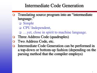
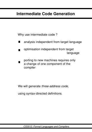
Intermediate Code Generation • Translating source program into an “intermediate language.” • Simple • CPU Independent, • …yet, close in spirit to machine language. • Or, depending on the application other intermediate languages may be used, but in general, we opt for simple, well structured intermediate forms. • (and this completes the “Front-End” of Compilation).
Types of Intermediate Languages • Graphical Representations. • Consider the assignment a:=b*-c+b*-c: assign assign a + + a * * * uminus b uminus uminus b b c c c
Syntax Dir. Definition for Gr. Reps. PRODUCTION Semantic Rule S id := E { S.nptr = mknode (‘assign’, mkleaf(id, id.entry), E.nptr) } E E1+ E2{E.nptr = mknode(‘+’, E1.nptr,E2.nptr)} E E1* E2{E.nptr = mknode(‘*’, E1.nptr,E2.nptr)} E - E1{E.nptr = mknode(‘uminus’, E1.nptr)} E ( E1 ) {E.nptr = E1.nptr } E id {E.nptr = mkleaf(id, id.entry)}
Three Address Code • Statements of general form x:=y op z • No built-up arithmetic expressions are allowed. • As a result, x:=y + z * wshould be represented ast1:=z * wt2:=y + t1x:=t2 • Observe that given the syntax-tree or the dag of the graphical representation we can easily derive a three address code for assignments as above. • In fact three-address code is a linearization of the tree. • Three-address code is useful: related to machine-language/ simple/ optimizable.
Example of 3-address code • t1:=- ct2:=b * t1t3:=- ct4:=b * t3t5:=t2 + t4a:=t5 • t1:=- ct2:=b * t1t5:=t2 + t2a:=t5
Types of Three-Address Statements. • x:=y op z • x:=op z • x:=z • goto L • if x relop y goto L • Push/pop (stack) more advanced: • param x1param x2…param xncall p,n • x:=&y x:=*y *x:=y • x:=y[i] x[i]:=y l-value of y (memory address That corresponds to variable y) Dereference of y, i.e., treat the r-value of y as memory Location and *y would be its Contents. Dereference of y+i, i.e. y[i] =df *(y+i)
Syntax-Directed Translation into 3-address code. • First deal with assignments. • Use attributes • E.place to hold the name of the “place” that will hold the value of E • Identifier will be assumed to already have the place attribute defined. • For example, the place attribute will be of the form t0, t1, t2, … for identifiers and v0,v1,v2 etc. for the rest. • E.code to hold the three address code statements that evaluate E (this is the `translation’ attribute). • Use function newtemp that returns a new temporary variable that we can use. • Use function gen to generate a single three address statement given the necessary information (variable names and operations).
Syntax-Dir. Definition for 3-address code PRODUCTION Semantic Rule S id := E { S.code = E.code||gen(id.place ‘=’E.place ‘;’) } E E1+ E2{E.place= newtemp ; E.code = E1.code || E2.code || || gen(E.place‘:=’E1.place‘+’E2.place) } E E1* E2{E.place= newtemp ; E.code = E1.code || E2.code || || gen(E.place‘=’E1.place‘*’E2.place) } E - E1{E.place= newtemp ; E.code = E1.code || || gen(E.place ‘=’ ‘uminus’ E1.place) } E ( E1 ) {E.place= E1.place ; E.code = E1.code} E id {E.place = id.entry ; E.code = ‘’} e.g. a := b * - (c+d)
What about things that are not assignments? • E.g. while statements of the form “while E do S”(intepreted as while the value of E is not 0 do S) Extension to the previous syntax-dir. Def. PRODUCTION S while E do S1 Semantic Rule begin = newlabel; after = newlabel ; S.code = gen(begin ‘:’) || E.code || gen(‘if’ E.place ‘=’ ‘0’ ‘goto’ after) || || S1.code || gen(‘goto’ begin) || gen(after ‘:’)
Dealing with Procedures P procedure ident ‘;’ block ‘;’ Semantic Rule begin = newlabel; Enter into symbol-table in the entry of the procedure name the begin label. P.code = gen(begin ‘:’) || block.code || gen(‘pop’ return_address) || gen(“goto return_address”) S call ident Semantic Rule Look up symbol table to find procedure name. Find its begin label called proc_begin return = newlabel; S.code = gen(‘push’return); gen(goto proc_begin) || gen(return “:”)
Implementations of 3-address statements • Quadruples t1:=- c t2:=b * t1 t3:=- c t4:=b * t3 t5:=t2 + t4 a:=t5
Implementations of 3-address statements, II • Triples t1:=- c t2:=b * t1 t3:=- c t4:=b * t3 t5:=t2 + t4 a:=t5
Other types of 3-address statements • e.g. ternary operations like x[i]:=y x:=y[i] • require two or more entries. e.g.
Implementations of 3-address statements, III • Indirect Triples
Declarations Using a global variable offset PRODUCTION Semantic Rule P M D { } M {offset:=0 } D id : T { addtype(id.entry, T.type, offset) offset:=offset + T.width } T char {T.type = char; T.width = 1; } T integer {T.type = integer ; T.width = 4; } T array [ num ] of T1 {T.type=array(1..num.val,T1.type) T.width = num.val * T1.width} T ^T1 {T.type = pointer(T1.type); T1.width = 4}
Keeping Track of Scope Information Consider the grammar fraction: P D D D ; D | id : T | proc id ; D ; S Each procedure should be allowed to use independent names. Nested procedures are allowed.
functions • Mktable(previous) creates a new symbol table and returns a pointer to the new table. previous points to the previously created symbol table. • enter(table, name, type, offset) creates a new entry for a name name in the symbol table pointed to by table • addwidth(table, witdth) • enterproc
Keeping Track of Scope Information (a translation scheme) P M D { addwidth(top(tblptr), top(offset)); pop(tblptr); pop(offset) } M { t:=mktable(null); push(t, tblptr); push(0, offset)} D D1; D2 ... D proc id ; N D ; S { t:=top(tblpr); addwidth(t,top(offset)); pop(tblptr); pop(offset); enterproc(top(tblptr), id.name, t)} N {t:=mktable(top(tblptr)); push(t,tblptr); push(0,offset);} D id : T {enter(top(tblptr), id.name, T.type, top(offset); top(offset):=top(offset) + T.width Example: proc func1; D; proc func2 D; S; S