Other Concept Classes
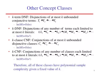
Other Concept Classes. k -term DNF: Disjunctions of at most k unbounded conjunctive terms: ln(| H |)=O( kn ) k -DNF: Disjunctions of any number of terms each limited to at most k literals: ln(| H |)=O( n k ) k -clause CNF: Conjunctions of at most k unbounded disjunctive clauses:

Other Concept Classes
E N D
Presentation Transcript
Other Concept Classes • k-term DNF: Disjunctions of at most k unbounded conjunctive terms: • ln(|H|)=O(kn) • k-DNF: Disjunctions of any number of terms each limited to at most k literals: • ln(|H|)=O(nk) • k-clause CNF: Conjunctions of at most k unbounded disjunctive clauses: • ln(|H|)=O(kn) • k-CNF: Conjunctions of any number of clauses each limited to at most k literals: • ln(|H|)=O(nk) Therefore, all of these classes have polynomial sample complexity given a fixed value of k.
Basic Combinatorics Counting Pick 2 from {a,b} All O(nk)
Expanded data with O(nk) new features Construct all disj. features with k literals Data for k-CNF concept k-CNF formula Find-S Computational Complexity of Learning • However, determining whether or not there exists a k-term DNF or k-clause CNF formula consistent with a given training set is NP-hard. Therefore, these classes are not PAC-learnable due to computational complexity. • There are polynomial time algorithms for learning k-CNF and k-DNF. Construct all possible disjunctive clauses (conjunctive terms) of at most k literals (there are O(nk) of these), add each as a new constructed feature, and then use FIND-S (FIND-G) to find a purely conjunctive (disjunctive) concept in terms of these complex features. Sample complexity of learning k-DNF and k-CNF are O(nk) Training on O(nk) examples with O(nk) features takes O(n2k) time
k-CNF Approximation Data for k-term DNF concept k-CNF Learner Enlarging the Hypothesis Space to Make Training Computation Tractable • However, the language k-CNF is a superset of the language k-term-DNF since any k-term-DNF formula can be rewritten as a k-CNF formula by distributing AND over OR. • Therefore, C = k-term DNF can be learned using H = k-CNF as the hypothesis space, but it is intractable to learn the concept in the form of a k-term DNF formula (also the k-CNF algorithm might learn a close approximation in k-CNF that is not actually expressible in k-term DNF). • Can gain an exponential decrease in computational complexity with only a polynomial increase in sample complexity. • Dual result holds for learning k-clause CNF using k-DNF as the hypothesis space.
Probabilistic Algorithms • Since PAC learnability only requires an approximate answer with high probability, a probabilistic algorithm that only halts and returns a consistent hypothesis in polynomial time with a high-probability is sufficient. • However, it is generally assumed that NP complete problems cannot be solved even with high probability by a probabilistic polynomial-time algorithm, i.e. RP ≠ NP. • Therefore, given this assumption, classes like k-term DNF and k-clause CNF are not PAC learnable in that form.
Infinite Hypothesis Spaces • The preceding analysis was restricted to finite hypothesis spaces. • Some infinite hypothesis spaces (such as those including real-valued thresholds or parameters) are more expressive than others. • Compare a rule allowing one threshold on a continuous feature (length<3cm) vs one allowing two thresholds (1cm<length<3cm). • Need some measure of the expressiveness of infinite hypothesis spaces. • The Vapnik-Chervonenkis (VC) dimension provides just such a measure, denoted VC(H). • Analagous to ln|H|, there are bounds for sample complexity using VC(H).
Shattering Instances • A hypothesis space is said to shatter a set of instances iff for every partition of the instances into positive and negative, there is a hypothesis that produces that partition. • For example, consider 2 instances described using a single real-valued feature being shattered by intervals. y x + –_ x,y x y y x x,y
Shattering Instances (cont) • But 3 instances cannot be shattered by a single interval. z y x + –_ x,y,z x y,z y x,z x,y z x,y,z y,z x z x,y x,z y Cannot do • Since there are 2m partitions of m instances, in order for H to shatter instances: |H| ≥ 2m.
VC Dimension • An unbiased hypothesis space shatters the entire instance space. • The larger the subset of X that can be shattered, the more expressive the hypothesis space is, i.e. the less biased. • The Vapnik-Chervonenkis dimension, VC(H). of hypothesis space H defined over instance space X is the size of the largest finite subset of X shattered by H. If arbitrarily large finite subsets of X can be shattered then VC(H) = • If there exists at least one subset of X of size d that can be shattered then VC(H) ≥ d. If no subset of size d can be shattered, then VC(H) < d. • For a single intervals on the real line, all sets of 2 instances can be shattered, but no set of 3 instances can, so VC(H) = 2. • Since |H| ≥ 2m, to shatter m instances, VC(H) ≤ log2|H|
VC Dimension Example • X: set of instances: points on the x, y plane • H: set of all linear decision surfaces in the plane • Any two distinct points can be shattered by H • VC(H)>=2 • For sets of three points, as long as they are not colinear, they can be shattered • VC(H)>=3 • No sets of size four can be shattered. VC(H)<4 • VC(H)=3 • H: any linear decision surfaces in an r dimensional space: VC(H)=r+1
VC Dimension Example • X: conjunction of exactly three boolean literals • H: the conjunction of up to three boolean literals • VC(H)?
VC Dimension Example • Consider axis-parallel rectangles in the real-plane, i.e. conjunctions of intervals on two real-valued features. Some 4 instances can be shattered. Some 4 instances cannot be shattered:
VC Dimension Example (cont) • No five instances can be shattered since there can be at most 4 distinct extreme points (min and max on each of the 2 dimensions) and these 4 cannot be included without including any possible 5th point. • Therefore VC(H) = 4 • Generalizes to axis-parallel hyper-rectangles (conjunctions of intervals in n dimensions): VC(H)=2n.
Upper Bound on Sample Complexity with VC • Using VC dimension as a measure of expressiveness, the following number of examples have been shown to be sufficient for PAC Learning (Blumer et al., 1989). • Compared to the previous result using ln|H|, this bound has some extra constants and an extra log2(1/ε) factor. Since VC(H) ≤ log2|H|, this can provide a tighter upper bound on the number of examples needed for PAC learning.
Conjunctive Learning with Continuous Features • Consider learning axis-parallel hyper-rectangles, conjunctions on intervals on n continuous features. • 1.2 ≤ length≤ 10.5 2.4 ≤ weight≤ 5.7 • Since VC(H)=2n sample complexity is • Since the most-specific conjunctive algorithm can easily find the tightest interval along each dimension that covers all of the positive instances (fmin ≤ f ≤ fmax) and runs in linear time, O(|D|n), axis-parallel hyper-rectangles are PAC learnable.
Sample Complexity Lower Bound with VC • There is also a general lower bound on the minimum number of examples necessary for PAC learning (Ehrenfeucht, et al., 1989): Consider any concept class C such that VC(H)≥2 any learner L and any 0<ε<1/8, 0<δ<1/100. Then there exists a distribution D and target concept in C such that if L observes fewer than: examples, then with probability at least δ, L outputs a hypothesis having error greater than ε. • Ignoring constant factors, this lower bound is the same as the upper bound except for the extra log2(1/ ε) factor in the upper bound.
COLT Conclusions • The PAC framework provides a theoretical framework for analyzing the effectiveness of learning algorithms. • The sample complexity for any consistent learner using some hypothesis space, H, can be determined from a measure of its expressiveness |H| or VC(H), quantifying bias and relating it to generalization. • If sample complexity is tractable, then the computational complexity of finding a consistent hypothesis in H governs its PAC learnability. • Constant factors are more important in sample complexity than in computational complexity, since our ability to gather data is generally not growing exponentially. • Experimental results suggest that theoretical sample complexity bounds over-estimate the number of training instances needed in practice since they are worst-case upper bounds.
COLT Conclusions (cont) • Additional results produced for analyzing: • Learning with queries • Learning with noisy data • Average case sample complexity given assumptions about the data distribution. • Learning finite automata • Learning neural networks • Analyzing practical algorithms that use a preference bias is difficult. • Some effective practical algorithms motivated by theoretical results: • Boosting • Support Vector Machines (SVM)
Mistake Bounds • So far, how many examples needed to learn? • What about: how many mistakes before convergence? • Let’s consider similar setting to PAC learning • Instances drawn at random from X according to distribution D • Learner must classify each instance before receiving correct classification from teacher • Can we bound the number of mistakes learner makes before converging?
Mistake bounds: Find-S • Consider Find-S when H=conjunction of boolean literals
Mistake Bounds: Halving Algorithm • Consider the Halving Algorithm • Learning concepts using version space candidate-elimination algorithm • Classify new instances by majority vote of version space members • How many mistakes before converging to correct H? • Worst case • Best case
Optimal Mistake Bounds • The lowest worst-case mistake bounds over all possible learning algorithms • Informally, the number of mistakes made for the hardest target concept in C, using the hardest training sequence.