Download
1 / 46
460 likes | 564 Vues
Explore exchange rate equilibrium, interest rate parity, and more in Chapter 5 of International Finance. Learn how to predict exchange rates and engage in profitable arbitrage opportunities.

E N D
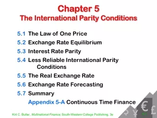
Chapter 5The International Parity Conditions 5.1 The Law of One Price 5.2 Exchange Rate Equilibrium 5.3 Interest Rate Parity 5.4 Less Reliable International Parity Conditions 5.5 The Real Exchange Rate 5.6 Exchange Rate Forecasting 5.7 Summary Appendix 5-A Continuous Time Finance
Prices Prices appear as upper case symbols Ptd = price of an asset at time t in currency d Std/f = spot exchange rate at time t in currency d Ftd/f = forward exchange rate between currencies d and f E[…] = expectation operator (e.g. E[St€/$])
Rates of change Changes in a price appear as lower case symbols rtd= an asset’s return in currency d during period t ptd= inflation in currency d in period t td= real interest rate in currency d in period t std/f = change in the spot rate during period t
The law of one price Equivalent assets sell for the same price (also called purchasing power parity, or PPP) • Seldom holds for nontraded assets • Can’t compare assets that vary in quality • May not hold precisely when there are market frictions
An example: The world price of gold Suppose P£ = £250/oz in London P€ = €400/oz in Berlin The law of one price requires: Pt£= Pt€ St£/€ Þ £250/oz = (€400/oz) (£0.6250/€) or 1/(£0.6250/€) = €1.6000/£ • If this relation does not hold, then there is an opportunity to lock in a riskless arbitrage profit.
An example with transactions costs Gold dealer AGold dealer B €401.40/oz Offer €401.00/oz Bid Sell high to B FX dealer €1.599/£ bid €1.601/£ ask Buy low from A £250.25/oz Offer £250.00/oz Bid
Cross exchange rate equilibrium Sd/e Se/f Sf/d = 1 If Sd/eSe/fSf/d < 1, then eitherSd/e, Se/f or Sf/d must rise ÞFor each spot rate, buy the currency in the denominator with the currency in the numerator If Sd/eSe/fSf/d > 1, then eitherSd/e, Se/f or Sf/d must fall ÞFor each spot rate, sell the currency in the denominator for the currency in the numerator
A cross exchange rate table £ C$ € ¥ SFr $ UK pound1.000 0.402 0.659 0.0052 0.451 0.622 Canadian $ 2.487 1.000 1.634 0.0130 1.120 1.546 Euro 1.518 0.612 1.000 0.0079 0.685 0.947 Japanese yen 191.6 77.24 126.1 1.0000 86.48 119.4 Swiss Franc 2.221 0.893 1.460 0.0116 1.000 1.381 US Dollar 1.609 0.647 1.057 0.0084 0.724 1.000
Cross exchange rates and triangular arbitrage Suppose SRbl/$ = Rbl 5.000/$ Û S$/Rbl= $0.2000/Rbl S$/¥ = $0.01000/¥ Û S¥/$ = ¥100.0/$ S¥/Rbl = ¥20.20/Rbl Û SRbl/¥» Rbl 0.04950/¥ SRbl/$ S$/¥ S¥/Rbl = (Rbl 5/$)($.01/¥)(¥20.20/Rbl) = 1.01 > 1
Cross exchange rates and triangular arbitrage SRbl/$ S$/¥ S¥/Rbl = 1.01 > 1 Þ Currencies in the denominators are too high relative to the numerators, so sell dollars and buy rubles sell yen and buy dollars sell rubles and buy yen
An example of triangular arbitrage SRbl/$ S$/¥ S¥/Rbl= 1.01 > 1 Sell $1 million and buy Rbl 5 million Sell ¥100 million yen and buy $1 million Sell Rbl 4.950 million and buy ¥100 million ÞProfit of 50,000 rubles = $10,000 at Rbls5.000/$ or 1% of the initial amount
International parity conditionsthat span both currencies and time Interest rate parityLess reliable linkages Ftd/f / S0d/f= [(1+id)/(1+if)]t = E[Std/f] / S0d/f = [(1+pd)/(1+pf)]t where S0d/f = today’s spot exchange rate E[Std/f] = expected future spot rate Ftd/f = forward rate for time t exchange i = a country’s nominal interest rate p = a country’s inflation rate
Interest rate parity Ftd/f/S0d/f = [(1+id)/(1+if)]t • Forward premiums and discounts are entirely determined by interest rate differentials. • This is a parity condition that you can trust.
Interest rate parity:Which way do you go? If Ftd/f/S0d/f > [(1+id)/(1+if)]t then so... Ftd/f must fall Sell f at Ftd/f S0d/f must rise Buy f at S0d/f id must rise Borrow at id if must fall Lend at if
Interest rate parity:Which way do you go? If Ftd/f/S0d/f < [(1+id)/(1+if)]t then so... Ftd/f must rise Buy f at Ftd/f S0d/f must fall Sell f at S0d/f id must fall Lend at id if must rise Borrow at if
Interest rate parity is enforced through “covered interest arbitrage” An Example: Given:i$ = 7% S0$/£ = $1.20/£ i£ = 3% F1$/£ = $1.25/£ F1$/£ / S0$/£> (1+i$) / (1+i£) 1.041667 > 1.038835 The fx and Eurocurrency markets are not in equilibrium.
Covered interest arbitrage +$1,000,000 1. Borrow $1,000,000 at i$ = 7% 2. Convert $s to £s at S0$/£ = $1.20/£ 3. Invest £s at i£ = 3% 4. Convert £s to $s at F1$/£ = $1.25/£ 5. Take your profit: Þ $1,072,920-$1,070,000 = $2,920 -$1,070,000 +£833,333 -$1,000,000 +£858,333 -£833,333 +$1,072,920 -£858,333
Forward rates as predictors of future spot ratesFtd/f = E[Std/f]or Ftd/f / S0d/f = E[Std/f] / S0d/f Forward rates are unbiased estimates of future spot rates.
Forward rates as predictors of future spot rates E[Std/f ] / S0d/f = Ftd/f / S0d/f Speculators will force this relation to hold on average • For daily exchange rate changes, the best estimate of tomorrow's spot rate is the current spot rate • As the sampling interval is lengthened, the performance of forward rates as predictors of future spot rates improves
Relative purchasing power parity (RPPP) Let Pt = a consumer price index level at time t Then inflation pt = (Pt - Pt-1) / Pt-1 E[Std/f] / S0d/f = (E[Ptd] / E[Ptf]) / (P0d /P0f) = (E[Ptd]/P0d) / (E[Ptf]/P0f) = (1+E[pd])t / (1+E[pf])t where pd and pf are geometric mean inflation rates.
Relative purchasing power parity (RPPP) E[Std/f] / S0d/f = (1+E[pd])t / (1+E[pf])t Speculators will force this relation to hold on average • The expected change in a spot exchange rate should reflect the difference in inflation between the two currencies. • This relation only holds over the long run.
International Fisher relation(Fisher Open hypothesis) [(1+id)/(1+if)]t = [(1+pd)/(1+pf)]t Recall the Fisher relation: (1+i) = (1+)(1+p) If real rates of interest are equal across currencies, then [(1+id)/(1+if)]t = [(1+d)(1+pd)]t / [(1+f)(1+pf)]t = [(1+pd)/(1+pf)]t
International Fisher relation (Fisher Open hypothesis) [(1+id)/(1+if)]t = [(1+pd)/(1+pf)]t Speculators will force this relation to hold on average • If real rates of interest are equal across countries (d =f ), then interest rate differentials merely reflect inflation differentials • This relation is unlikely to hold at any point in time, but should hold in the long run
International Fisher relation Difference in realized quarterly inflation Difference in 3-month interest rates
Summary: Int’l parity conditions International Fisher relation Interest rates [(1+id)/(1+if)]t Inflation rates [(1+pd)/(1+pf)]t Interest rate parity Relative PPP Ftd/f / S0d/f Forward-spot differential E[Std/f] / S0d/f Expected change in the spot rate Forward rates as predictors of future spot rates
The real exchange rate • The real exchange rate adjusts the nominal exchange rate for differential inflation since an arbitrarily defined base period
Change in the nominal exchange rate Example S0¥/$ = ¥100/$ S1¥/$ = ¥110/$ E[p¥] = 0% E[p$] = 10% s1¥/$ = (S1¥/$–S0¥/$)/S0¥/$ = 0.10, or a 10 percent nominal change
The expected nominal exchange rate But RPPP implies E[S1¥/$] = S0¥/$ (1+ p¥)/(1+ p$) = ¥90.91/$ What is the change in the nominal exchange rate relative to the expectation of ¥90.91/$?
Actual versus expected change St¥/$ ¥130//$ ¥120//$ ¥110//$ Actual S1¥/$ = ¥110/$ ¥100//$ E[S1¥/$] = ¥90.91/$ ¥90//$ time
Change in the real exchange rate • In real (or purchasing power) terms, the dollar has appreciated by (¥110/$) / (¥90.91/$) - 1 = +0.21 or 21 percent more than expected
Change in the real exchange rate (1+xtd/f) = (Std/f / St-1d/f) [(1+ptf)/(1+ptd)] where xtd/f = percentage change in the real exchange rate Std/f = the nominal spot rate at time t ptc = inflation in currency c during period t
Change in the real exchange rate ExampleS0¥/$ = ¥100/$ S1¥/$ = ¥110/$ E[p¥] = 0% and E[p$] = 10% xt¥/$ = [(¥110/$)/(¥100/$)][1.10/1.00] -1 = 0.21, or a 21 percent increase in real purchasing power
Behavior of real exchange rates • Deviations from purchasing power parity • can be substantial in the short run • and can last for several years • Both the level and variance of the real exchange rate are autoregressive
Real value of the dollar (1970-1998) Mean level = 100 for each series
Appendix 5-AContinuous time finance • Most theoretical and empirical research in finance is conducted in continuously compoundedreturns
Holding period returnsare asymmetric r1 =+100% r2 =-50% 200 100 100 (1+rTOTAL) = (1+r1)(1+r2) = (1+1)(1-½) = (2)(½) = 1 rTOTAL = 0%
Continuous compounding Let r = holding period (e.g. annual) return r = continuously compounded return r = ln (1+r) = ln (er) Û (1 + r) = er where ln(.) is the natural logarithm with base e » 2.718
Continuous returns are symmetric +69.3% -69.3% 200 100 100 rTOTAL = Ln[(1+r1)(1+r2)] = r1+r2 = +0.693 - 0.693 = 0.000 rTOTAL = 0%
Properties of natural logarithms(for x > 0) eln(x) = ln(ex) = x ln(AB) = ln(A) + ln(B) ln(At) = t * ln(A) ln(A/B) = ln(AB-1) = ln(A) - ln(B)
Continuously compounded returns are additiverather than multiplicative ln[ (1+r1) (1+r2) ... (1+rT) ] = r1 + r2 +... + rT
The international parity conditionsin continuous time Over a single period ln(F1d/f /S0d/f ) = id– if = E[pd ]– E[pf ] = E[sd/f ] where s d/f, p d, p f, i d, and i f are continuously compounded
The international parity conditionsin continuous time Over t periods ln(Ftd/f /S0d/f ) = t(id– if ) = t(E[pd ]– E[pf ]) = tE[sd/f ] where s d/f, p d, p f, i d, and i f are continuously compounded