Download
1 / 29
310 likes | 657 Vues
Momentum Heat Mass Transfer. MHMT 7. Turbulent flows.

E N D
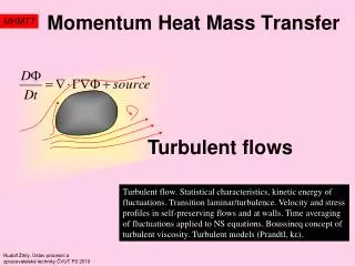
Momentum Heat Mass Transfer MHMT7 Turbulent flows Turbulent flow. Statistical characteristics, kinetic energy of fluctuations. Transition laminar/turbulence. Velocity and stress profiles in self-preserving flows and at walls. Time averaging of fluctuations applied to NS equations. Boussineq concept of turbulent viscosity. Turbulent models (Prandtl, k). Rudolf Žitný, Ústav procesní a zpracovatelské techniky ČVUT FS 2010
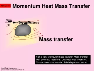
NS equations and Turbulence The convection term is a quadratic function of velocities – source of nonlinearities and turbulent phenomena MHMT7 Navier Stokes equations are nonlinear even in the case that the viscosity is constant. Primary source of nonlinearities in the Navier Stokes equations are convective inertial terms Relative magnitude of inertial (nonlinear) and viscous (linear) terms is Reynolds number
Turbulence Distarbunce is attenuated Distarbunce is amplified MHMT7 Increasing Re increases nonlinearity of NS equations. This nonlinearity leads to sensitivity of NS solution to flow disturbances. Laminar flow: Re<Recrit Turbulent flow: Re>Recrit Velocity field (controlled by NS equations) depends on boundary and initial conditions. Let us assume steady boundary conditions (time independent velocity/pressure profiles at inlets/outlets): There will be only one (or two) steady solutions in the laminar flow regime, independent of initial conditions (starting velocity field). On the other hand the flow field will be unsteady and depending upon initial conditions (sometimes will be sensitive even to infinitely small disturbances) in the turbulent flow regime.
Turbulence - fluctuations MHMT7 Turbulence can be defined as a deterministic chaos. Velocity and pressure fields are NON-STATIONARY (du/dt is nonzero) even if flowrate and boundary conditions are constant. Trajectory of individual particles are extremely sensitive to initial conditions (even the particles that are very close at some moment diverge apart during time evolution). Velocities, pressures, temperatures… are still solutions of NS and energy equations, however they are non-stationary and form chaotically oscillating turbulent vortices (eddies). Time and spatial profiles of transported properties are characterized by fluctuations Actual value at given time and space Mean value fluctuation
Turbulence fluctuations MHMT7 • Statistics of turbulent fluctuations • Mean values (remark: mean values of fluctuations are zero) • rms (root mean square) • Kinetic energy of turbulence • Intensity of turbulence • Reynolds stresses
Turbulent eddies - scales MHMT7 Kinetic energy of turbulent fluctuations is the sum of energies of turbulent eddies of different sizes Large energetic eddies (size L) break to smaller eddies. This transformation is not affected by viscosity E() Spectral energy of turbulent eddies Inertial subrange (inertial effects dominate and spectral energy depends only upon wavenumber and ) Smallest eddies (size is called Kolmogorov scale) disappear, because kinetic energy is converted to heat by friction =2f/u 1/L 1/ wavenumber (1/size of eddy) Typical values of frequency f~10 kHz, Kolmogorov scale ~0.01 up to 0.1 mm Kolmogorov scale decreases with the increasing Re
Turbulent eddies - scales MHMT7 Kolmogorov scales (the smallest turbulent eddies) follow from dimensional analysis, assuming that everything depends only upon the kinematic viscosity and upon the rate of energy supply in the energetic cascade (only for small isotropic eddies, of course) velocity scale Time scale Length scale These expressions follow from dimension of viscosity [m2/s] and the rate of energy dissipation [m2/s3]
Transition laminar-turbulent MHMT7 There always exists a steady solution of NS equation corresponding to the laminar flow regime, but need not be the only one. Sometimes even an infinitely small disturbance is enough for a jump to unsteady turbulent regime, sometimes the disturbance must by sufficiently strong (typical for viscous instabilities). Therefore the transition from laminar to turbulent flow regime cannot be always specified by a unique Recrit because it depends upon the level of disturbances (laminar flow can be achieved in pipe at Re10000 in laboratory). Hopper
Transition laminar-turbulent Inflection – source of instability (max.gradient) y velocity y velocity MHMT7 • Hydrodynamic instabilities are classified as • Inviscid instabilities characterised by existence of inflection point of velocity profile - jets - wakes - boundary layers wit adverse pressure gradient p>0 • Viscous instabilities • Linear eigenvalues analysis (Orr-Sommerfeld equations) • - channels, simple shear flows (pipes) • - boundary layers with p>0 Poiseuille flow ~ 5700 Couette flow – stable? There is no inflection of velocity profile in a pipe, however turbulent regime exists if Re>2100
Transition laminar-turbulent MHMT7 • How to indentify whether the flow is laminar or turbulent ? • Experimentally Visualization, hot wire anemometers, LDA (Laser Doppler Anemometry). • Numerical experiments Start numerical simulation selected to unsteady laminar flow. As soon as the solution converges to steady solution for sufficiently fine grid the flow regime is probably laminar • Recrit According to the value of Reynolds number using literature data of critical Reynolds number
Transition laminar-turbulent D D D D D D D/2 D MHMT7
Jets and mixing layer umax u b h y u y umin MHMT7 Free flows (self preserving flows) Jets Mixing layers Wakes umax Jet thickness ~x, mixing length ~x see Goertler, Abramovic Teorieja turbulentnych struj, Moskva 1984: x Circular jet Planar jet x
Turbulence at walls MHMT7 Flow at walls (boundary layers) y Friction velocity Log law Buffer layer Laminar sublayer u INNER layer (independent of bulk velocities) OUTER layer (law of wake)
Turbulence at walls MHMT7 Flow at walls (turbulent stresses) t Prandtl’s model vanDriest model of mixing length lm 5 30
Time averaging fluctuation MHMT7 RANS (Reynolds Averaging of Navier Stokes eqs.) Time average Favre’s average Proof: Remark: Favre’s average differs only for compressible substances and at high Mach number flows. Ma>1
Time averaging fluctuation MHMT7 Continuity equation Navier Stokes equations Reynolds stresses
Time averaging fluctuation MHMT7 Fourier Kirchhoff, mass transport, kinetic energy equations for transport of scalars Turbulent fluxes
Turbulent viscosity MHMT7 It was Boussinesq who suggested: Why not to calculate the turbulent Reynolds stresses and turbulent heat fluxes in the same way like in laminar flows, just replacing actual viscosity by an artificially increased turbulent viscosity and to replace actual driving potential (rate of deformation) by driving potential evaluated from averaged velocities, temperatures,… this is self portrait of Hopper …and this is Joseph Boussinesq
Turbulent viscosity MHMT7 Analogy to Fourier law Analogy to Newton’s law Rate of deformation based upon gradient of averaged velocities
Turbulent viscosity - models h h y MHMT7 Prandtl’s model of mixing length. Turbulent viscosity is derived from analogy with gases, based upon transport of momentum by molecules (kinetic theory of gases). Turbulent eddy (driven by main flow) represents a molecule, and mean path between collisions of molecules is substituted by mixing length. Excellent model for jets, wakes, boundary layer flows. Disadvantage: it fails in recirculating flows (or in flows where transport of eddies is very important). u(y) Circular jet Planar jet Mixing length Mixing layers Currently used algebraic models are Baldwin Lomax, and Cebecci Smith
Turbulent viscosity - models MHMT7 • Two equation models calculate turbulent viscosity from the pairs of turbulent characteristics k-, or k-, or k-l (Rotta 1986) • k (kinetic energy of turbulent fluctuations) [m2/s2] • (dissipation of kinetic energy) [m2/s3] (specific dissipation energy) [1/s] Wilcox (1998) k-omega model, Kolmogorov (1942) Jones,Launder (1972), Launder Spalding (1974) k-epsilon model C = 0.09 (Fluent-default)
Turbulent viscosity - models MHMT7 Standard k- model Transport equation for kinetic energy of turbulence (see also lecture 9) production term (energy of main flow converted to energy of turbulent eddies) convective transport diffusive transport by fluctuating turbulent eddies dissipation kinetic energy of turbulence to heat Similar transport equation for dissipation of kinetic energy this term follows from inspection analysis
CFD modelling - FLUENT MHMT7 This is example of 2 pages in Fluent’s manual (Fluent is the most frequently used program for Computer Fluid Dynamics modelling)
EXAM MHMT7 Turbulence
What is important (at least for exam) MHMT7 Definition of turbulence – deterministic chaos (stability of solution of NS equations, explain role of convective acceleration) Statistical characteristics (what is it the second correlation?) Kinetic energy Intensity of turbulence Reynolds stresses
D D D D What is important (at least for exam) MHMT7 Transition laminar-turbulent flows. Critical Reynolds number 10 2100 500000 400
What is important (at least for exam) MHMT7 Velocity profile at wall u+(y+) (how to calculate w?) Friction velocity Laminar sublayer y+<5
What is important (at least for exam) MHMT7 Boussinesq hypotheses of turbulent viscosity (what is the difference between and ?) Prandtl’s model of turbulent viscosity (what is it lm?) Principles of k-epsilon models. Derive turbulent viscosity as a function of k and .