Parallel Computing
Parallel Computing. Michael Young, Mark Iredell. NWS Computer History. 1968 CDC 6600 1974 IBM 360 1983 CYBER 205 first vector parallelism 1991 Cray Y-MP first shared memory parallelism 1994 Cray C-90 ~16 gigaflops 2000 IBM SP first distributed memory parallelism 2002 IBM SP P3

Parallel Computing
E N D
Presentation Transcript
Parallel Computing Michael Young, Mark Iredell
NWS Computer History • 1968 CDC 6600 • 1974 IBM 360 • 1983 CYBER 205 first vector parallelism • 1991 Cray Y-MP first shared memory parallelism • 1994 Cray C-90 ~16 gigaflops • 2000 IBM SP first distributed memory parallelism • 2002 IBM SP P3 • 2004 IBM SP P4 • 2006 IBM SP P5 • 2009 IBM SP P6 • 2013 IBM Idataplex SB ~200 teraflops NEMS/GFS Modeling Summer School
Algorithm of the GFS Spectral Model • One time loop is divided into : • Computation of the tendencies of divergence, surface pressure, temperature and vorticity and tracers (grid) • Semi-implicit time integration (spectral) • First half of time filter (spectral) • Physical effects included in the model (grid) • Damping to simulate subgrid dissipation (spectral) • Completion of the time filter (spectral) NEMS/GFS Modeling Summer School
Algorithm of the GFS Spectral Model Definitions : Operational Spectral Truncation T574 with a Physical Grid of 1760 longitudes by 880 latitudes and 64 vertical levels (23 km resolution) θ is latitude λis longitude l is zonal wavenumber n is total wavenumber (zonal + meridional) NEMS/GFS Modeling Summer School
Three Variable Spaces • Spectral (L x N x K) • Fourier (L x J x K) • Physical Grid ( I x J x k) I is number of longitude points J is number of latitudes K is number of levels NEMS/GFS Modeling Summer School
The Spectral Technique All fields possess a spherical harmonic representation: where NEMS/GFS Modeling Summer School
Spectral to Grid Transform Legendre transform: Fourier transform using FFT: NEMS/GFS Modeling Summer School
Grid to Spectral Transform Inverse Fourier transform (FFT): Inverse Legendre (Gaussian quadrature): NEMS/GFS Modeling Summer School
MPI and OpenMP • GFS uses Hybrid 1-Dimensional MPI layout and OpenMP threading at do loop level • MPI (Message Passing Interface) is used to communicate between tasks which contain a subgrid of a field • OpenMP supports shared memory multiprocessor programming (threading) using compiler directives NEMS/GFS Modeling Summer School
MPI and OpenMP • Data Transposes are implemented using MPI_alltoallv • Required to switch between the variable spaces which have different 1-D MPI decompositions NEMS/GFS Modeling Summer School
Spectral to Physical Grid • Call sumfln_slg_gg (Legendre Transform) • Call four_to_grid (FFT) • Data Transpose after Legendre Transform in preparation for FFT to Physical grid space call mpi_alltoallv(works,sendcounts,sdispls,mpi_r_mpi, x workr,recvcounts,sdispls,mpi_r_mpi, x mc_comp,ierr) NEMS/GFS Modeling Summer School
Physical Grid to Spectral • Call Grid_to_four (Inverse FFT) • Call Four2fln_gg (Inverse Legendre Transform) • Data Transpose performed before the Inverse Legendre Transform call mpi_alltoallv(works,sendcounts,sdispls,MPI_R_MPI, x workr,recvcounts,sdispls,MPI_R_MPI, x MC_COMP,ierr) NEMS/GFS Modeling Summer School
Physical Grid Space Parallelism • 1-D MPI distributed over latitudes. OpenMP threading used on longitude points. • Each MPI task holds a group of latitudes, all longitudes, and all levels • Cyclic distribution of latitudes used for load balancing the MPI tasks due to a smaller number of longitude points per latitude as latitude increases (approaches the poles). NEMS/GFS Modeling Summer School
Physical Grid Space Parallelism • Cyclic distribution of latitudes example 5 MPI tasks and 20 Latitudes would be Task 1 2 3 4 5 Lat 1 2 3 4 5 Lat 10 9 8 7 6 Lat 11 12 13 14 15 Lat 20 19 18 17 16 NEMS/GFS Modeling Summer School
Physical Grid Space Parallelism Physical Grid Vector Length per OpenMPthread • NGPTC (namelist variable) defines number (block) of longitude points per group (vector length per processor) that each thread will work on • Typically set anywhere from 15-30 points NEMS/GFS Modeling Summer School
Spectral Space Parallelism • Hybrid 1-D MPI layout with OpenMP threading • Spectral space 1-D MPI distributed over zonal wave numbers (l's). OpenMP threading used on a stack of variables times number of levels. • Each MPI task holds a group of l’s, all n’s, and all levels • Cyclic distribution of l's used for load balancing the MPI tasks due to smaller numbers of meridional points per zonal wave number as the wave number increases. NEMS/GFS Modeling Summer School
GFS Scalability • 1-D MPI scales to 2/3 of the spectral truncation. For T574 about 400 MPI tasks. • OpenMP threading scales to 8 threads. • T574 scales to 400 x 8 = 3200 processors. NEMS/GFS Modeling Summer School