Download

1 / 49
620 likes | 1.05k Vues
스케줄 이론 Baker's Ch. 10 Flow Shop Scheduling. 1. Introduction. Characteristics of Flow shop problem ① Each job consists of several operations following linear precedence relationships.

E N D
스케줄 이론 Baker's Ch. 10 Flow Shop Scheduling
1. Introduction • Characteristics of Flow shop problem • ① Each job consists of several operations following linear precedence relationships. • ② Each operation can be done on one and only one machine in a shop (If not, it can be combined logically ). • ③ Operations of every job follow the same flow pattern. • 1:1 relationship between machines and operations. • We can number the machines according to the flow pattern.
1. Introduction • (Terminology) • ① Pure flow shop: Every machine is used in every job. • ② General flow shop: Not every machine is used in every job even though the flow pattern is maintained • Without loss of generality, we can treat them as the same class of problems assuming = 0 for not visited machines, where is the processing time of the job i, operation(machine) j
1. Introduction • Assumptions • ① All jobs are available at time 0. • ② Sequence independent set up time. • ③ Job descriptors known. • ④ No machine-down time. • ⑤ No preemption. • Complete enumeration • n! possible sequence for each machine (m machine) • (Digression) • Assembly line, Kanban: They seek "even processing time" while maintaining permutation schedule only.
m1 1 2 m2 1 2 m3 1 2 m3 1 2 14 m1 2 1 (b) m2 2 1 m3 2 1 m3 2 1 14 1. Introduction • One difference: Inserted idle time F1=1+5 F2=4*2+1 F3=4*2+1 F4=1*2+4 (a) m1 1 2 (c) m2 1 2 Idle time m3 2 1 m3 2 1 12
Suppose jobs i, j M/C 1 (i,1) (j,1) M/C 2 (j,2) (i,2) Cj Ci ... No change in completion times 2. Permutation schedules • Permutation schedules • Single machine : Permutation schedule is enough. • Job shop : Much larger classes of schedules should be considered. • Flow shop : In between single machine and job shop problems. In some cases, permutation schedule is enough. • (Theorem 1) • To minimize regular measure of performance, we need consider only schedules in which the same job sequence is followed on the first 2 machines. • (Sketch of the proof) : Gantt Chart • The operation (j,2) can not start before the completion time of (j,1). By interchanging (i,1) and (j,1), we lose nothing for the regular measure of performance. But now (j,2) may possibly be started earlier.
Suppose jobs i, j M/C m-1 (i,m-1) (j,m-1) M/C m (j,m) (i,m) Cj Ci ... No change in completion times 2. Permutation schedules • (Theorem 2) • In Min. makespan problem, we need consider only schedules in which the same job sequence is followed on the last 2 machines. • (Proof) • We lose nothing as far as makespan is concerned. But earlier processing is possible for operations (i,m) and (j,m) because (j,m) was bounded by (j,m-1). • Using Theorems 1 and 2, permutation schedule is enough for following cases. • ① Regular measure m = 2. • ② Makespan m = 3.
2. Permutation schedules • But still, it is not easy to find an optimum schedule (Permutation schedule is still n!). And Theorem 2 does not hold for regular measure of performance in general. • (Counter Example) 2 job, 3 M/C flow shop problem, . • Job Descriptors or but
3. The Two-Machine Problem • 3.1. Johnson's problem • Finding an optimum schedule for n job, 2-machine (permutation schedule) flow shop problem with minimize makespan criterion. • (Algorithm 1) Johnson's Algorithm • 1. Find job j such that holds. • 2. If the Minimum happened to be M/C 1, then put j in the first position. Otherwise put j in the last position. • 3. Exclude j from further consideration and go to STEP 1. • (Example) • (Algorithm 2) Implementing Johnson’s Rule (sets U={j| aj ≤ bj } and V ={j| aj > bj }
3. The Two-Machine Problem • (Discussion) • Consider lower bounds for the makespan M. Since there are only two machines, let for convenience. Then, • To reduce lower bounds, choose smallest • The idea is intuitively appealing but it is not clear whether it gives us an optimal. • The contribution of Johnson's algorithm is two fold: the theorem itself and the elegance of the proof (A classic example of standardized proof). • The so-called Johnson's rule refers to the following rule. • In an optimal sequence for M, following holds for two jobs "i" and "j" : • Johnson's algorithm would give us an optimal solution for two algorithms if above rule is true and transitive.
3. The Two-Machine Problem • 3.2 Proof of Johnson's rule • Since there are only two machines, machine idleness (that causes longer makespan) occurs only on M/C 2 (Jobs on M/C 1 can be compacted).
3. The Two-Machine Problem • Consider S which does not obey Johnson's order. • Let S' be a schedule with i & j interchanged. • Now consider , where B is the set of jobs preceding i & j. • Add Q on both sides of ①, especially
3. The Two-Machine Problem • (Proof of transitivity)
Baker’s 2nd Edition • In a rigorous sense, transitivity may not hold if there are ties. For a single machine case, we were indifferent to tie breaking mechanisms, and we obtained optimal in any way. But here, we are not indifferent when ties occur. • In the book, Baker illustrates an example where adjacent pairs satisfy Johnson’s inequality but non-adjacent pairs do not. • However, our algorithms 1 and 2 all generate the optimal solutions for the make span problem.
3.3, 3.4 Variations to Two Machine Problem • (Terminology) Lap phasing (Lap scheduling) • A portion of a job moved & worked on next M/C before completion of work in previous M/C (Lot splitting allowed). • Start Lag (= aj) is defined to be the time that M/C 2 can start job j after the start of job j on M/C 1. • Stop Lag (= bj) is defined to be the time that M/C 2 can not finish job j after the completion of job j on M/C 1, that is M/C 2 can not finish before . • In Mitten's original paper(1959), aj = bj ≈ Dj
3.3, 3.4 Variations to Two Machine Problem • (Algorithm) Mitten's algorithm • 2 machine, Min. makespan flow shop problem with start and stop lags. • (Step 1) Let • (Step 2) Sequence the jobs in U with non-decreasing , sequence jobs in V with non –increasing . • (e.g.) • But, Mitten's algorithm is optimum only on permutation schedules, and it works on m machine flow shop problems when only the first machine(the machine 1) and the last machine(machine m) are the bottleneck machines.
4. Three M/C Makespan problem • (Fact) Permutation schedule is enough. But no general constructive algorithm (e.g. Johnson's) exists. • Constructive algorithm works only for special cases. • (e.g.) • Case 1. Machine 1 dominates machine 2: • Operation times for machine 2 are dominated by machine 1 or machine 3. • Then set (pseudo two-machine problem) and apply Johnson's method(called the Johnson's approximate method). • Case 2. Machine 3 dominates machine 2: • Johnson’s approximate method • Case 3. Regressive second stage: • Johnson’s approximate method • Case 4. Machine 2 dominates machine 1: • 먼저 m/c 2, 3의 two machine problem을 먼저 푼다. 여기서 job k를 첫번째 job이라고 하면 1번기계에서 job k 작은 processing time을 가지는 job 을 맨 앞에 두는 스케줄들을 만들어 이 중에서 가장 작은 makespan을 가지는 것이 three-machine에서의 optimal이 된다. • Case 5. Machine 2 dominates machine 3:
4. Three M/C Makespan problem • Case 6. Johnson’s extended rule • Three 2 M/C sub-problems yield the same permutation schedule. • Case 7. Constant second stage: • Machine 1의 SPT schedule과 Machine 3의 LPT schedule이 동일하면 optimal임 • Case 8. Lower bound condition for Johnson’s approximate method • M: makespan corresponding to an optimal sequence to the pseudoproblem of Johnson’s approximate method • M': actual makespan in the three-machine problem for the same sequence • This sequence is optimal if
4. Three M/C Makespan problem • Then what happens when we use Johnson's rule as a heuristic algorithm. • The experimental result of Wagner & Giglio: • (They applied Johnson's rule to 20 test problems setting ) • 9 optimal, 8 very close to optimal (by simple pair-wise interchange we can get to the optimal). On the average, solutions 3 % over optimal. • In conclusion, Johnson's algorithm works pretty good for 3 machine flow shop problems. • The experimental result of Smits and Baker(1981) • Approximately about half of the problems meets the condition(Cases 1-8) to find the optimal. • Generated 900 test problems( Random: Ordered: Constant 2nd: Correlated: Trend: Correlated-Trend) x 50 x (5, 20, 50 jobs) • Case 8 accounted for most of the success.
5. Minimizing the Makespan • 5.1 Branch and Bound Solution • B & B (1965, O.R. : the following two papers appeared almost at the same time) • (Ignall and Schrage ) and (Lomnicki) • Min M for flowshop - Optimal for m 3 (it generated permutation schedules)
Ignall-Schrage algorithm • Let us call the set of partially sequenced jobs and the set of unscheduled jobs ′. • And let q1 = Completion time for jobs in for M/C 1 • q2 = Completion time for jobs in for M/C 2 • q3 = Completion time for jobs in for M/C 3, • then the lower bounds based on M/C 1's completion time becomes • And the LB based on M/C 2's completion time is • And the LB based on M/C 3's is • Finally the LB for partial sequence is B = Max{b1, b2, b3}
5. Minimizing the Makespan • (Property) F1 • Suppose contain the same jobs in different order. And, • need not be considered any further in the search for an optimum
5. Minimizing the Makespan • Extensions to Original B & B Algorithm Refined Bounds • (Brown and Lomnicki, ORQ, 1966) where b2′is obtained by q2′and b3′is obtained by q3′ . M/C 3
5. Minimizing the Makespan • McMahon & Burton's Extension. (1967, O.R.): Job-based bound • They claimed that previous bounds were all machine based bounds (say, the completion times at the machines). • We need to spend throughput times for the jobs in ’, once we finish all jobs in . • Divide ′ into such that
5. Minimizing the Makespan • The combination of machine-based and job-based bounds represented by B′ will lead to a more efficient search of the branching tree in the sense that fewer nodes will be created.
5. Minimizing the Makespan • Some considerations on B&B methods for 3 M/C Flow Shop Problem • ① The tighter the LB is, the smaller the size of the solution tree. (especially so for the case of jump tracking) • ② It should be easy to calculate the LB (We need to balance ① and ②) • ③ The efficiency of branching procedure depends on the data. Especially, if the lower bounds of two un-branched nodes have the same value, which one should be selected next? • In general, we follow the job with a lower job number, and according to the experiment of McMahon and Burton, assigning job numbers according to increasing ti1 sequence works better (say assign job numbers according to SPT sequence). • ④ Reduction of branching is possible by the Dominance Property.
5. Minimizing the Makespan • And for 3 M/C cases, we can use reversed problem. • Permutation schedule is enough. • Construction of a reversed problem. • (e.g.) 1-2-3 ⇒ 3-2-1 • (Makespan is the same(?) for any flow shop problem.) • Conditions (by experience) where reversed problem leads to less branching • Experimental result shows that for large problems( n≥7, m=3), saving is significant.
5. Minimizing the Makespan • 5.2 Heuristic Approaches to Makespan Problems • The performance comparison of heuristic solutions that consider only permutation schedules for the n job m machine makespan problems.
5. Minimizing the Makespan • ① Palmer's algorithm (1965) • (Idea) Observations from Johnson's algorithm. • (1) The jobs that appear in the front in optimum schedule are the jobs that have longer processing times at later machines. • (2) The jobs that appear in the back in optimum schedule are the jobs that have shorter processing times at later machines. • Assign indexes for each job. • The index values are designed such that the jobs may have higher values if it has longer processing times at later machines ⇒ Assign jobs with higher values to the front in a schedule. • Slope index Sj • Let • Then the permutation schedule is . • According to the experiments conducted on 1580 problems( n≤6, m≤10 ), we found optimum for about 30% of the cases(Based on Dannenbring, 1977, Mgt. Science. V.23, pp1174-1182)
5. Minimizing the Makespan • ② Gupta's Algorithm(1972) • (Idea) Further observation on Johnson's Algorithm. • For the case of 3 machine problems with , we could use Johnson's Algorithm by modifying the problem to two machine problem by • For such cases, we get an optimum permutation schedule for 3 M/C case if we set the Index • So for the case of m machines, let • Then set schedule with non-increasing sj sequence.
5. Minimizing the Makespan • ③ Capmbell, Dudek & Smith(1970)'s: • Sometime called the "CDS" Heuristic • Recall that applying Johnson's Algorithm blindly to 3 m/c problem as if it were a 2 m/c problem with worked as a good heuristic. • CDS Algorithm is an extension of such method. Say, we convert n job m machine problem into (m-1) sub-problems and then select the best one among these (m-1) schedules. • Say, set , then apply Johnson's 2 m/c Algorithm • According to Dannenbring's experiment(1977), the algorithm found optimal solutions for 55% of cases for 1580 problem sets. Furthermore, the possibility of finding an optimal solution is large by a simple neighborhood search method(say, from 1, 2, 3, ..., n, we get 2, 1, 3, ..., n or 1, 3, 2, ..., n)
5. Minimizing the Makespan • ④ Dannenbring's Algorithm(1977, Mgt. Science. V.23, pp1174-1182) • Using the result of observations on Johnson's Algorithm • If we set this way, then have small values if the processing times at earlier machines are small, and have small values if the processing times at later machines are small. • Now apply Johnson's 2 m/c Algorithm + (n-1) neighborhood search after then. • Stop when no improvement is possible. • Found optimal in 75% of the cases for 1580 test problems. But CDS is 10 times faster than Dannenbring's.
5. Minimizing the Makespan • ⑤ Nawaz, Enscore & Ham, "A Heuristic Search Algorithm for the m m/c, n-job flow shop sequencing problem," OMEGA, InJMS(1983). • ⑥ Booth & Turner, "Comparison of Heuristics for Flow Shop Sequencing," OMEGA, InJMS(1987).
5. Minimizing the Makespan • ⑦ Widmer & Hertz, "A New Heuristic Method for the Flow Shop Sequencing Problem," EJOR(1989). • (Idea) • a) Distance between jobs a,b, a measure of increase in makespan if a precedes b. • Say we assign high penalty for the difference in processing times at earlier machines. • STEP 1: Find a, b such that , then set a to precede b. • STEP 2: Repeat STEP 1 until all jobs are scheduled. (Choose next job arbitrarily) • b) Then apply Taboo search : Pair-wise interchange. (not necessarily adjacent)
5. Minimizing the Makespan • Extension of Johnson's Algorithm for NON-FLOW SHOP(2 Machine Job Shop) • Let A = {All jobs which run only on m/c 1} • B = {All jobs which run only on m/c 2} • AB = {All jobs which run on m/c 1 then m/c 2} • BA = {All jobs which run on m/c 2 then m/c 1} • The Procedure • (1) Apply Johnson's Algorithm to A, B, AB. • (2) Arbitrarily order for A, B. • (3) Then run each machine as follows. • M/C 1: AB, A, BA • M/C 2: BA, B, AB • The procedure above generates optimum solution for Min MAKESPAN problem of 2 machine job shop problem. • (Why?) Consider m/c idle time. • M/C 2 is kept idle waiting for jobs of type AB • M/C 1 is kept idle waiting for jobs of type BA • The schedule minimizes such idle time.
6. Variations of the M-machine Model • Flow Shops without Intermediate Queues • No waiting at machines in the middle once a job started (Steel mills, Heat treatment, Casting and Forging). • The problem can be reduced to Traveling Salesman Problem Branch & Bound.
6. Variations of the M-machine Model • Min problem • (1) 2 M/C case • Fact 1) Johnson's Algorithm does not work (not even generally good). • Fact 2) For 2 job, 2 M/C problem. • For regular measures, we need consider only permutation schedules. Consider
6. Variations of the M-machine Model • Theorem: ① is satisfied when • (proof) • The condition is sufficient. • (e.g.)
6. Variations of the M-machine Model • Fact 3) N job 2 M/C problem • i) need consider only permutation schedules (N!) • ii) no idle in M/C 1 • iii) for any 2 adjacent jobs, results of FACT2) may be used. But the condition is sufficient & transitivity has not been proven. • Fact 4) Ignall & Schrage B & B • Lower bound for total flow time = where, • Say, SPT rule applied only on . • The computational complexity is (better than n!) • Also the optimal for n-1 job problem contributes nothing for n job problem.
6. Variations of the M-machine Model • (2) Min in n Job m machine flow shop problem • B & B (Bansal, 1977, IIE Trans.) • Lower Bound (Undetermined) (Constant)
6. Variations of the M-machine Model • Let ... ① ... ② ... ③
6. Variations of the M-machine Model • (B & B ALGORITHM) • STEP 1: Find lower bound for n job(n node) using ① (σ = 1) • STEP 2: Branch to smallest LB and determine (n-1) LB's • STEP 3: Branch to smallest LB among all nodes still unfathomed (jump-tracking) • STEP 4: Continue B & B. If tie occurs among unbranched nodes, branch with greater |σ| • (Discussion) • ① Min & Min M gives different solution. • ② We consider only Permutation Schedules.
6. Variations of the M-machine Model • Integer Programming for Permutation Schedules (by Wagner, Story & Giglio) • Let
6. Variations of the M-machine Model • Min Minimizing Idle Time on M/C 3 • # of Iterations( Using Gomory's Algorithm ) Complete Permutation • Practically No Use. • B & B seems the best approach.
7. Summary • Permutation Schedule is enough for • 3 M/C, Makespan problems • 2 M/C, Regular measure problems • Makespan : • 2 M/C: Johnson's algorithm • Non-Preempt, 3 M/C: NP-Complete Garey et al. (1976) (Maths of O.R.) • Preempt, 3 M/C: NP-Complete Gonzalez & Sahni (1978) ( O.R. ) • B & B. Lageweg, Lenstra, Rinnooy Kan, 1978, O.R. • Not easy to find solutions if the number of processor is over 5. • Heuristic: CDS, Dannenbring, Neh, (Booth & Turner), (Nawze, Euscere, Ham), (Widmar & Hertz) • Mean Flow Time: B & B by Bansal • T problem: YD Kim(1993)