Introduction to Algorithms Dynamic Programming – Part 2
Introduction to Algorithms Dynamic Programming – Part 2. CSE 680 Prof. Roger Crawfis. The 0/1 Knapsack Problem. Given: A set S of n items, with each item i having w i - a positive weight b i - a positive benefit Goal: Choose items with maximum total benefit but with weight at most W.

Introduction to Algorithms Dynamic Programming – Part 2
E N D
Presentation Transcript
Introduction to Algorithms Dynamic Programming – Part 2 CSE 680 Prof. Roger Crawfis
The 0/1 Knapsack Problem • Given: A set S of n items, with each item i having • wi - a positive weight • bi - a positive benefit • Goal: Choose items with maximum total benefit but with weight at most W. • If we are not allowed to take fractional amounts, then this is the 0/1 knapsack problem. • In this case, we let Tdenote the set of items we take • Objective: maximize • Constraint:
Example • Given: A set S of n items, with each item i having • bi - a positive “benefit” • wi - a positive “weight” • Goal: Choose items with maximum total benefit but with weight at most W. “knapsack” Items: box of width 9 in 1 2 3 4 5 • Solution: • item 5 ($80, 2 in) • item 3 ($6, 2in) • item 1 ($20, 4in) Weight: 4 in 2 in 2 in 6 in 2 in Benefit: $20 $3 $6 $25 $80
First Attempt • Sk: Set of items numbered 1 to k. • Define B[k] = best selection from Sk. • Problem: does not have sub-problem optimality: • Consider set S={(3,2),(5,4),(8,5),(4,3),(10,9)} of(benefit, weight) pairs and total weight W = 20 Best for S4: Best for S5:
Second Attempt • Sk: Set of items numbered 1 to k. • Define B[k,w] to be the best selection from Sk with weight at most w • This does have sub-problem optimality. • I.e., the best subset of Sk with weight at most w is either: • the best subset of Sk-1 with weight at most w or • the best subset of Sk-1 with weight at most w-wk plus item k
Knapsack Example item weight value 1 2 $12 2 1 $10 3 3 $20 4 2 $15 Knapsack of capacity W = 5 w1 = 2, v1=12 w2 = 1, v2=10 w3 = 3, v3=20 w4 = 2, v4=15
Algorithm • Since B[k,w] is defined in terms of B[k-1,*], we can use two arrays of instead of a matrix. • Running time is O(nW). • Not a polynomial-time algorithm since W may be large. • Called a pseudo-polynomial time algorithm. Algorithm01Knapsack(S,W): Input:set S of n items with benefit biand weight wi; maximum weight W Output:benefit of best subset of S with weight at most W letAandBbe arrays of lengthW + 1 forw 0to W do B[w]0 fork 1 to n do copy arrayBinto arrayA forwwkto Wdo ifA[w-wk] +bk > A[w]then B[w]A[w-wk] +bk returnB[W]
Longest Common Subsequence (LCS) • A subsequence of a sequence/string S is obtained by deleting zero or more symbols from S. For example, the following are some subsequences of “president”: pred, sdn, predent. In other words, the letters of a subsequence of S appear in order in S, but they are not required to be consecutive. • The longest common subsequence problem is to find a maximum length common subsequence between two sequences.
LCS For instance, Sequence 1: president Sequence 2: providence Its LCS is priden. president providence
LCS Another example: Sequence 1: algorithm Sequence 2: alignment One of its LCS is algm. a l g o r i t h m a l i g n m e n t
Naïve Algorithm • For every subsequence of X, check whether it’s a subsequence of Y . • Time:Θ(n2m). • 2msubsequences of X to check. • Each subsequence takes Θ(n)time to check: scan Y for first letter, for second, and so on.
Optimal Substructure Notation: prefix Xi= x1,...,xiis the first iletters of X. Theorem Let Z = z1, . . . , zk be any LCS of X and Y . 1. If xm= yn, then zk= xm= ynand Zk-1 is an LCS of Xm-1 and Yn-1. 2. If xmyn, then either zkxmand Z is an LCS of Xm-1 and Y . 3. or zkynandZ is an LCS of X and Yn-1.
Optimal Substructure Proof:(case 1: xm= yn) Any sequence Z’ that does not end in xm= yncan be made longer by adding xm= ynto the end. Therefore, • longest common subsequence (LCS) Z must end in xm= yn. • Zk-1 is a common subsequence of Xm-1 and Yn-1, and • there is no longer CS of Xm-1 and Yn-1, or Z would not be an LCS. Theorem Let Z = z1, . . . , zk be any LCS of X and Y . 1. If xm= yn, then zk= xm= ynand Zk-1 is an LCS of Xm-1 and Yn-1. 2. If xmyn, then either zkxmand Z is an LCS of Xm-1 and Y . 3. or zkynandZ is an LCS of X and Yn-1.
Optimal Substructure Proof: (case 2: xmyn, andzkxm) Since Z does not end in xm, • Z is a common subsequence of Xm-1 and Y, and • there is no longer CS of Xm-1 and Y, or Z would not be an LCS. Theorem Let Z = z1, . . . , zk be any LCS of X and Y . 1. If xm= yn, then zk= xm= ynand Zk-1 is an LCS of Xm-1 and Yn-1. 2. If xmyn, then either zkxmand Z is an LCS of Xm-1 and Y . 3. or zkynandZ is an LCS of X and Yn-1.
Recursive Solution • Define c[i, j] = length of LCS of Xiand Yj. • We want c[m,n].
Recursive Solution c[springtime, printing] c[springtim, printing] c[springtime, printin] [springti, printing] [springtim, printin] [springtim, printin] [springtime, printi] [springt, printing] [springti, printin] [springtim, printi] [springtime, print]
Recursive Solution • Keep track of c[a,b] in a table of nm entries: • top/down • bottom/up
How to compute LCS? • Let A=a1a2…am and B=b1b2…bn . • len(i, j): the length of an LCS between a1a2…ai and b1b2…bj • With proper initializations, len(i, j) can be computed as follows.
The Backtracking Algorithm procedure Output-LCS(A, prev, i, j) • if i = 0 or j = 0 then return • if prev(i, j)=”“ thenOutput-LCS(A, prev, i-1, j-1) Print A[i]; • else if prev(i, j)=”“ thenOutput-LCS(A, prev, i-1, j) • else Output-LCS(A, prev, i, j-1)
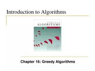
Transitive Closure • Compute the transitive closure of a directed graph • If there exists a path (non-trivial) from node i to node j, then add an edge to the resulting graph. • Also called the reachability: If a can reach b and b can reach c, then a can reach c. From Wikipedia.org: http://en.wikipedia.org/wiki/File:Transitive-Closure.PNG
Warshall’sAlgorithm • On the kth iteration, the algorithm determines for every pair of vertices i, j if a path exists from i and j with just vertices 1,…,k allowed as intermediate nodes. R(k-1)[i,j] (path using just 1 ,…,k-1) R(k)[i,j] = or R(k-1)[i,k] and R(k-1)[k,j] (path from i to k and from k to j using just 1 ,…,k-1) { k i Initial condition? j
3 3 1 1 4 4 2 2 Warshall’s Algorithm • Constructs transitive closure T as the last matrix in the sequence of n-by-n matrices R(0), … , R(k), … , R(n) where • R(k)[i,j] = 1 iff there is nontrivial path from i to j with only the first k vertices allowed as intermediate • Note that R(0) = A (adjacency matrix), R(n) = T (transitive closure) • Example: Path’s with only node 1 allowed.
3 3 3 3 3 1 1 1 1 1 4 2 4 4 2 2 4 4 2 2 Warshall’s Algorithm • Complete example: R(0) 0 0 1 0 1 0 0 1 0 0 0 0 0 1 0 0 R(1) 0 0 1 0 1 01 1 0 0 0 0 0 1 0 0 R(2) 0 0 1 0 1 0 1 1 0 0 0 0 1 1 1 1 R(3) 0 0 1 0 1 0 1 1 0 0 0 0 1 1 1 1 R(4) 0 0 1 0 1 1 1 1 0 0 0 0 1 1 1 1
3 1 4 2 3 1 4 2 Warshall’sAlgorithm 0 0 1 0 1 0 0 1 0 0 0 0 0 1 0 0 0 0 1 0 1 0 1 1 0 0 0 0 0 1 0 0 R(0) = R(1) = 0 0 1 0 1 0 1 1 0 0 0 0 1 1 11 0 0 1 0 1 1 1 1 0 0 0 0 1 1 1 1 0 0 1 0 1 0 1 1 0 0 0 0 1 1 1 1 R(2) = R(4) = R(3) =
Warshall’sAlgorithm Time efficiency: Θ(n3) Space efficiency: Matrices can be written over their predecessors (with some care), so it’s Θ(n2).