Download

1 / 29
290 likes | 397 Vues
This session aims to equip participants with the skills to analyze consumption patterns using SPSS and STATA. The focus is on understanding how monthly per capita food expenditure is influenced by education levels and gender of household heads. We will cover the procedures for entering data into SPSS, performing a two-way ANOVA, and interpreting results, including testing for assumptions like homogeneity of variances. Participants will learn to identify significant differences in expenditure patterns based on gender and education, and how to perform follow-up analyses for significant interactions.

E N D
Consumption Pattern : SPSS/STATA SrinivasuluRajendran Centre for the Study of Regional Development (CSRD) Jawaharlal Nehru University (JNU) New Delhi India r.srinivasulu@gmail.com
Objective of the session To understand consumption pattern through software packages
1. How to Analyze consumption pattern? 2. What are procedure available for estimating consumption pattern and how to do with Econometric software
Two-way ANOVA using SPSS • The two-way ANOVA compares the mean differences between groups that have been split on two independent variables (called factors). You need two independent, categorical variables and one continuous, dependent variable .
Objective • We are interested in whether an monthly per capita food expenditure was influenced by their level of education and their gender head. Monthly per capita food expenditure with higher value meaning a better off. The researcher then divided the participants by gender head of HHs i.e Male head & Female head HHs and then again by level of education.
In SPSS we separated the HHs into their appropriate groups by using two columns representing the two independent variables and labelled them “Head_Sex" and “Head_Edu". For “head_sex", we coded males as "1" and females as “0", and for “Head_Edu", we coded illiterate as "1", can sign only as "2" and can read only as "3“ and can read & write as “4”. Monthly per capita food expenditure was entered under the variable name, “pcmfx".
How to correctly enter your data into SPSS in order to run a two-way ANOVA
Testing of Assumptions • In SPSS, homogeneity of variances is tested using Levene's Test for Equality of Variances. This is included in the main procedure for running the two-way ANOVA, so we get to evaluate whether there is homogeneity of variances at the same time as we get the results from the two-way ANOVA.
Perform the two-anova test procedure which is explained in the previous session.
Tests of Between-Subjects Effects Table • The table shows the actual results of the two-way ANOVA as shown • We are interested in the head of hhs gender, education and head_sex*head_edu rows of the table as highlighted above. These rows inform us of whether we have significant mean differences between our groups for our two independent variables, head_sex and head_edu, and for their interaction, head_sex*head_edu. We must first look at the head_sex*head_edu interaction as this is the most important result we are after. We can see from the Sig. column that we have a statistically NOT significant interaction at the P = .686 level. You may wish to report the results ofhead_sex and head_edu as well. We can see from the above table that there was no significant difference in monthly per capita food exp between head_sex (P = .675) but there were significant differences between educational levels (P < .000).
We can see from the table that there is some repetition of the results but, regardless of which row we choose to read from, we are interested in the differences between (1) illiterate, (2) can sign, (3) can read, (4) can read & write. From the results we can see that there is a significant difference between selected different combinations of educational level (P < .0005).
Homogeneous Subsets Overall, both subset shows insignificant, there was no homogeneous among subsets
The following plot is not of sufficient quality to present in your reports but provides a good graphical illustration of your results. In addition, we can get an idea of whether there is an interaction effect by inspecting whether the lines are parallel or not.
From this plot we can see how our results from the previous table might make sense. Remember that if the lines are not parallel then there is the possibility of an interaction taking place.
Procedure for Simple Main Effects in SPSS • You can follow up the results of a significant interaction effect by running tests for simple main effects - that is, the mean difference in monthly per capita food expenditure between head of gender HHs at each education level. SPSS does not allow you to do this using the graphical interface you will be familiar with, but requires you to use syntax.
You will be presented with the Syntax Editor as shown below: • Type text into the syntax editor so that you end up with the following (the colours are automatically added): • [Depending on the version of SPSS you are using you might have suggestion boxes appear when you type in SPSS-recognised commands, such as, UNIANOVA. If you are familiar with using this type of auto-prediction then please feel free to do so, but otherwise simply ignore the pop-up suggestions and keep typing normally
UNIANOVA pcmfx BY head_sexhead_edu • /EMMEANS TABLES(head_sex*head_edu) COMPARE(head_sex)
Basically, all text you see above that is in CAPITALS, is required by SPSS and does not change when you enter your own data. Non-capitalised text represents your variables and will change when you use your own data. Breaking it all down, we have:
Making sure that the cursor is at the end of row 2 in the syntax editor click the button, which will run the syntax you have typed. Your results should appear in the Output Viewer below the results you have already generated.
This table shows us whether there are statistical differences in mean monthly per capita food expenditure between head of gender for each educational level. We can see that there are no statistically significant mean differences between male and females' headed HHs in pcmfx when head of HHs are educated to illetrate (P = .785) or can sign (P = .718) so on.
You should emphasize the results from the interaction first, before you mention the main effects. In addition, you should report whether your dependent variable was normally distributed for each group and how you measured it (we will provide an example below). • A two-way ANOVA was conducted that examined the effect of head of gender and education level on per capita monthly food expenditure. There was no homogeneity of variance between groups as assessed by Levene's test for equality of error variances. There was a no significant interaction between the effects of head of gender and education level on per capita monthly food expenditure, F =0.377, P = .686. Simple main effects analysis showed that male headed HH were NOT significantly different in monthly per capita food expenditure than female headed HH when educated to read & write, but there were differences in monthly per capita food expenditure when the head of HHs educated to read & write (P = .000), However, there was no significant different between male head and female head HHs in pcmfx.
Hands-on Exercises 1. Find out whether an monthly per capita total expenditure was influenced by their gender head and districts. 2. Find out whether an monthly per capita total expenditure was influenced by the village those who adopted technology and districts.