Microsoft Excel 2000

1. Microsoft Excel 2000 Lecture 1

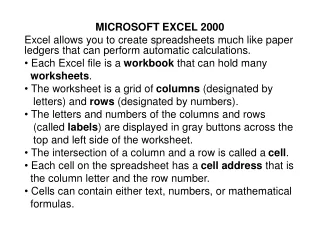
2. Overview of Excel • Excel is a spreadsheet program. • Excel is used to analyse numerical data. • Excel replaces the function of a calculator. • You can enter and format data easily. • You can analyse data by using formulas and functions. • You can view data as a graph or chart. • You can make what-if analysis.

3. Loading Excel 2000 • Click START Menu. • Choose Programs. • Choose Microsoft Excel.

4. Introducing Excel Window

5. Control-menu buttons are restore,move, size, minimize, maximize, close. Minimize, Restore and Close buttons. Titlebar displays program name and filename. Workspace displays workbook window Standard Toolbar Formula Bar Edit Formula Button Menubar Name Box Format Toolbar Status Bar

6. Workbook Window • Displays a new blank workbook file containing three blank sheets. • A sheet is used to display different types of information, such as financial data or charts. • Whenever you open a new workbook it displays a worksheet. • A worksheet, also referred as spreadsheet is a rectangular grid of rows and columns used to enter data. It is the primary type of sheet you will use in excel. • The parts of the worksheet are...

7. Introducing Workbook Window

8. Cell Selector identifies active cell. Active Sheet Tab Scroll Buttons Row Column Column Letters Row Numbers

9. Name box displays reference of Active Cell. Formula box displays the value of Active Cell.

10. Using the Office Assistant • You can use the office assistant as in MS Word. • Press F1 to display office assistant. • Then you can type your question and display the related help topics as usual.

11. Using Toolbars • Standard and Formatting toolbars are displayed automatically. • Standard toolbar contains most frequently used buttons. • Buttons on the formatting toolbar are used to change the format and the design of the worksheets. • You can open toolbars by using View Toolbars... Menu item.

12. Moving around the Worksheet • Either the MOUSE or the KEYBOARD can be used to move CELL SELECTOR from one cell to another.

13. Moving with Keyboard •  move left •  move right •  move up •  move down • Page-up move one page up • Page-down move one page down • CTRL+  last column • CTRL+  last row

14. Entering Data

15. Types of Entries • The information you enter in a cell can be: • TEXT • NUMBERS • FORMULAS

16. Text Entries • Can contain any combination of letters, numbers, spaces, and any other special characters. • Max 32000 characters can be entered in a cell. • By default they are aligned to left.

17. Number Entries • Number entries can contain only the digits 0 to 9 and any of the special characters + - ( ) , . / $ % E e. • Number entries are used in calculations. • Numbers are aligned to right, by default.

18. Formula Entries • An entry that begins with an equal sign “=“ is a formula. • Formula entries perform calculations using numbers or data contained in other cells. The resulting value is a variable value because it can change if the data it depends changes. • In contrast a number value is a constant value.

19. Entering Data Example

20. Text entries are LEFT Aligned. Cell Selector moves down after you press ENTER. Goto B2 and press “J” character. You can use cancel and enter buttons to cancel the entry or complete the entry with your mouse. Type “anuary” to complete the word to “January” and press ENTER. You can press BACKSPACE if you have mistyped a character. Active CELL displays Entry and Insertion Point Let’s Enter Data CANCEL BUTTON ENTER BUTTON Formula Bar Displays Entry

21. Enter Edit Delete Copy: Data

22. Insertion Point Numeric entries are right aligned by default. Now A6 cannot be displayed completely, but it is displayed completely in the formula bar. Long text Entry. DELETE key deletes the next character to the I-Beam. • Position insertion point to end of the word January. • Press BACKSPACE6 times. • Type “AN”. • Press Enter button. BACKSPACE key deletes the previous character to the I-Beam. Mouse pointer is now an I-beam. You can position insertion point by using mouse as well. You can move insertion point by using HOME, END, , keys. Then These: B6 94000 C6 89000 D6 120000 E6 145000 F6 125000 G6 125000 Write following: C5 135000 D5 200000 E5 210000 F5 185000 G5 185000 Now write row headings: A4SALES A5Clothing A6Hard Goods A7Total Sales Moving horizontally write the words FEB, MAR, APR, MAY, JUN and TOTAL in cells C3 through H3. Let’s Edit the Contents of the cell B3 and changeJanuary to JAN. • Put your mouse over cell B3. • Double click or press F2. • Move to B5 • Type140000 • Press Save the workbook with the name “Sales Data” Move to C2 and type “1999 First Half Budget” You should have a similar looking worksheet. ENTERING NUMBERS

23. Now enter Expenses Data. Then select cells C13 to G15 and press paste again. CUT, COPY, PASTE SHORT-CUTS CUT CTRL+X COPYCTRL+C PASTECTRL+V • Move to cell B5 • Enter =B5+C5+D5+E5+F5+G5 • Press ENTER. If you change the contents of one of the cells B5 to G5 then formula is recalculated. Then copy contents of B12 to C12 by using Copy & Paste buttons. Now select cells through D12 to G12 and press paste. ENTERING FORMULAS Now select cells B13 to B15 and copy cells. Results of the calculation appears in the cell.

24. Data formats in Excel include: General, Number Currency, Accounting Date, Time Percentage, Fraction Scientific,Text Special, Custom You can change the format of cells using FormatCells... Menu item. You can change Data Format, Alignment, Fonts, Borders, Background, from this dialog box.

25. Previewing and Printing Worksheets

26. Preview FilePrint Preview... Print FilePrint... Previewing and Printing an Excel Workbook

27. Select cells through B10 to G10. • Type =B7*4% • Press CTRL+Enter Again we observe that the correct versions of the formulas are entered to all of the selected cells. Now Enter the formula =B7*58% to the cells in range B11 to G11 using same method. • Move to B7 • Type = • Select B5 • Press + • Select B6 • Press Enter Command Formulas B7*4%, C7*4%, ... G7*4% are entered automaticly. Notice that the formula in B7 =B5+B6 changes relative to the cell it is copied. It becomes =C5+C6 in C7. You can copy the formulas in the same way as other values. Copy the formula in B7 to cells C7 to G7 using range-selection. Write formulas using print mode Formula =B5+B6 is calculated in cell B7

28. Range references blank cells. Press Autosum button. Function Name Range Argument Range is corrected. Press Enter Command. • Now • Goto cell B18 and select the range B18 to G18. • Then Enter formula =B7-B16 • ress CTRL+Enter. Using functions you can increase your Productivity. You can write =SUM(B10:B15) instead of the formula B10+B11+B12+B13+B14+B15 Entering Functions Excel proposes a range to automaticly for you. Now Press Enter command and enter formula. Now copy the function from B16 to range C16 to G16. Move to cell B16. Copy cell H6 to range H7 to H18. Obsreve result. Goto H6 and press Autosum button. Excel proposals incorrect range. Now select range B6 to G6 Move to H8

29. Name Box as drop down list Dialog-box reduced to a single bar to allow easy access to worksheet. Proposed Argument Range Hide dialog box to select range. Press Paste Function Button • Because the proposed argument list is incorrect, (it includes total) we will select the actual range. • ClickHide Dialog Box button. Press Restore Dialog box button. Description of function Restores display of dialog box. Press OK. Formula Result Calculated • SelectStatistical • Then Average • Press OK Select B5 through G5 Copy the function to cells I5 to I18. • Move to I3. • TypeAVG and right align it. • Move to I5. Another way to enter a function is Paste Function utility.

30. Enter comment to text box. Red triangle indicates cell has a comment. Comment text box name PressEnterCommand when it shows $H$7 reference. To view the commentagain point to cell or select View Commentsmenu item. To clarify the meaning of cell contents you can enter a comment to a cell. From Insert menu selectComment • Reference types • H7Relative reference. • $H$7Absolute reference. • $H7Mixed reference. • H$7Mixed reference. If you continue to pressF4 you will observe all kind of references. ($H$7, $H7, H$7, H7). What we wanted was to compute ratio H6/H7. So H7 must be an absolute reference rather than a relativereference. To close the commentclickanywhere outside the comment box. After copying J5 to J6observe on the formula bar that H7referencedoesn’t change. • Move to J5. • Enter=H5/H7 To get ratio of sale to total sales. Type“Total hard goods sales as a percent of total sales” as comment. Goto J5 and pressF2 to edit it. Error occurs because formula becomes H6/H8 Move cursor to start of H7 and press F4. Copy cell to J6.

31. Changing the column width

32. Column A contains many interrupted headings. Reference Line shows the place of the moving column width. Column Width The size or width of a column controls how much information can be displayed in a cell. A text entry that is longer than the column width will be fully displayed only if the cells to the right are blank. If the cells contains data, then the text is interrupted. The column width can be quickly adjusted by dragging the column divider line located to the right of the column letter. Dragging it to the right increases column width. Max column width is 255. Drag the column divider line located to the right of the column letter. All the cells in the selected columns have changed to five character spaces. Notice that a series of number signs (#####) appears in most of the worksheet cells. Whenever the width of a cell is too small to display the entire number, number signs are displayed. Next you want to see how the columns would be displayed if you decrease the width of all the columns from B to J. You can decrease the width of all the columns individually, but there is a faster way to do this. Now you can set the width of all columns by setting the width of one of the selected columns. Just repeat the previous step. And then goto A1. After entering the numbers for January in column B, any long headings in column A were cut off or interrupted. To allow the long text entries to be fully displayed, you can increase the column’s width. To set the width of multiple columns you should select the columns you want by clicking the first one and then dragging your mouse. As you can see, this new column width is too small. To cancel the most recent operation and restore the worksheet to how it was prior to your change Click UNDO. The effects of the column width setting are reversed to the prior column width setting. To undo several actions at once, open the Undo drop-down list and select the actions you want to reverse. All actions above the selected actions are also reversed. Adjusting Column Widths

33. Zooming the worksheet

34. You can reduce or enlarge the amount of information displayed onscreen by changing the magnification from between 10 to 400 percent. You want to display more information: Open zoom drop-down menu. Select 75%.

35. Formatting Numbers • Number format affect how numbers look on screen when they are printed. They do not affect how excel stores or uses the values in calculations. • The default format setting that controls how numbers are displayed in worksheet is General. • General automatically sets the number format to a Date, Time, Comma, Currency, Percent or Scientific number format depending on the characters you used when entering data.

36. continued... • The table below shows samples of how Excel automatically formats a number based on how it appears when you enter it. ENTRY FORMAT 10,000 Comma $102.20 Currency with 2 decimal places. 90% Percent with zero decimal places. 10/30/98 Date 9:10 Time

37. continued... • If no symbol is used, Excel leaves the number unformatted. • Unformatted numbers are displayed without a thousand separator such as comma, with negative values preceded by a – (minus sign), and with as many decimal place settings as the cell space allows.

38. Click decrease decimal places button 2 times. A quick way of selecting a range is to select the first cell of the range then press Shift key and then pressing the last key of the range. You will change the number format of cells through B5 to I18 to display dollar signs, commas, and decimal places. Click OK. AutoFit feature automatically adjusts column width to display the contents of cells within the selection. Using this method select the range B5 through I18. Then Select Format/Column/AutoFit Menu Item. A second category that displays number as currency is accounting. If necessary open the number tab and select currency. Click format cells.

39. Cell Alignment

40. Select cells from A5 to A7 and A10 to A16 by using CTRL key. Observe that the contents of the selected cells are indended 2 levels. Now open Format/Cells and select Alignment tab. This time we will set Left alignment and Indentation level to 2. You can set cell alignment to any item in this drop-down box.

41. Inserting rows

42. You may want to insert rows after filling some parts of the worksheet. You may do this by choosing Insert/Rows. You may also insert columns by choosing Insert/Columns. Goto A3 and Select Insert/Rows item from the menu bar.

43. Centering Across a Selection

44. Press Merge and Center button on format toolbar. You may want to set a heading for your workbook, visible on the workbook. Select cells from A2 to I2 Lets make our heading at C3 centered.

45. Changing Fonts and Font Styles

46. Select Times New Roman from font-face drop down list. Click Bold. Select 12 from font size drop-down list. You want to improve the worksheet appearence by enhancing the appearance of the title. To do this you can change the font settings. Double-click format painter. Click A10 and A19. Click format painter. Font settings are common to all Office family of programs. Now select range B6 to I19. Change format to Accounting from Format/Cells... Then select Format/Columns/AutoFit Selection... Move to A5. Press Bold and Italic. Finally, you want to bold and underline the column headings. Select B4 through I4. Click bold and underline. Set row heading in A8 and A17 to Bold.

47. Adding Headers and Footers

48. Select Setup... Select Header/Footer tab. Open Header list and select your name, date, page number option. You can select a predefined footer by the same method. To add a header, Preview the worksheet using File/Print Preview.

49. Changing Page Orientation

50. Now press previous and then choose setup. Now you can print spreadsheet by using the print command. To see second page click next. Dont forget to set page tab. Then choose landscape option. You can use landscape style to fit the contents of worksheet on the same paper. Notice that entire page does not fit on the screen.