1995 “Sunrise Fire ” Westhampton , NY Image taken from the Cutchogue Fire Department web

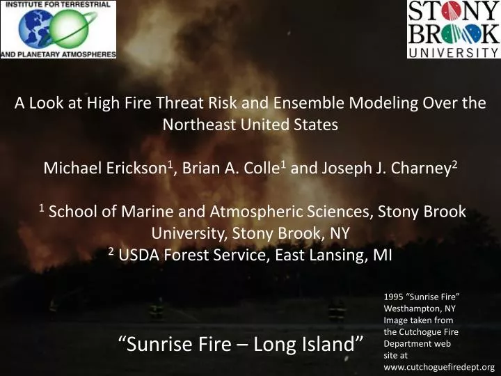
1. A Look at High Fire Threat Risk and Ensemble Modeling Over the Northeast United StatesMichael Erickson1, Brian A. Colle1 and Joseph J. Charney21 School of Marine and Atmospheric Sciences, Stony Brook University, Stony Brook, NY2 USDA Forest Service, East Lansing, MI 1995 “Sunrise Fire” Westhampton, NY Image taken from the Cutchogue Fire Department web site at www.cutchoguefiredept.org “Sunrise Fire – Long Island”

2. Wildfires and the Northeast United States • A wildfire is any uncontrolled fire in combustible vegetation and can grow to enormous sizes. • Wildfires are natural occurrences, but they can also be destructive to humans and the ecosystem. • The sustenance and spread of wildfires is VERY sensitive to the overlying meteorology conditions (i.e. dryness, wind speed, direction, temperature, etc). • Although rare, wildfires along the Northeast coast of the United States can be dangerous due to a high population density. United States Forest Service 2010

3. Ridge-Manorville Brush Fire – April 9th, 2012 • 1000-2000 acres burned. • 600 firefighters from 109 departments battled the fire with 30 brush trucks, 20 tankers and 100 engines. • New York State Police Helicopters made airdrops of water. • Fortunately the fire broke out in a relatively rural area of Long Island. Source: longislandpress.com Source: newsday.com Source: new12.com

4. Sunrise Fire – late August 1995 • 7000 acres burned by a series of brush fires between late August and early September. • Highways and railways were closed cutting off the Hamptons from the rest of Long Island. • Numerous homes and business were damaged, as was the pine barrens ecosystem. Source: pb.state.ny.us Source: pb.state.ny.us Source: dmna.ny.gov

5. Forecasting Wildfire Occurrence 100-Hour Fuel Moisture (10/4/12) • Attempts to forecast wildfire occurrence are relatively new, and based both on the surface conditions and overlying atmosphere. • Many fire-risk parameters consider the current state of vegetation, fuel moisture, local meteorology and terrain height. • There is still the additional complex factor that many wildfires are caused by human activity. Lower Atmosphere Haines Index (10/4/12) Fire Danger Class (10/4/12)

6. All days with high fire threat risk should be examined, since similar ground/weather conditions may not always produce a fire due to human influences. • Model performance on high fire threat days should be known if model output is going to be used to drive high fire threat forecasts. • Model biases may vary with the atmospheric flow pattern on high fire threat days, suggesting potential room for improvement in model post-processing. Motivation Goals • Define a High Fire Threat Index (HFTI) that captures the occurrence and strength of fire threat risk between 1979-2012. • Evaluate model performance and post-processing methods on high fire threat days compared to the typical warm season day. • Determine if meteorological model biases vary with “weather regime” and suggest ways this can be used to improve operational forecasts.

7. Fuels (i.e. dead leaves/brush) for wildfires dry out quickly, and can occur within a day of a rain event if atmospheric conditions are favorable. • Relative humidity is the main driver for forest fires, while wind speed is a secondary driver. • Considering fire threat over a smaller regional area is desirable since it increases the sample size while ensuring the region considered has relatively homogenous weather conditions. Defining High Fire Threat Strength (HFTS) - Assumptions Source: longislandpress.com

8. The Automated Surface Observing System (ASOS) station observations shown to the right are used between 1979-2012. • HFTS Definition • No rainfall > 0.5” or snow cover at any station 24 hours before the high fire threat day starts. • HFTS consists of 5 categories; a total of 3 categories from relative humidity (RH) and two from wind speed (WS). • Mean daytime RH must be in the bottom 2.5, 1, and 0.5 percentile to achieve sub-categories 1, 2, and 3, respectively. • If RH criteria is meet, WS > 10 and 15 knots are needed to meet the WS criteria for sub-categories 1 and 2, respectively. • HFTS consists of summing the RH and WS components and can vary between 0 and 5. High Fire Threat Strength (HFTS)- Definition Relative Humidity Hrly Histogram Arrows indicate bottom 0.5, 1, and 2.5 percentile, respectively

9. Fire Threat Frequency by Month Fire Threat Frequency by Month Fire Threat Frequency by Year Fire Threat – Monthly and Annual Variability • High fire threat days typically occur between March and May, and may have been increasing in frequency more recently.

10. Fire Threat Frequency by Year - Relative Humidity Component Only Fire Threat Frequency by Year - Wind Speed Component Only Fire Threat – Annual Variability • The recent increase in high fire threat risk is caused mostly by drier rather than windier conditions.

11. Analyzed the National Center For Environmental Prediction (NCEP) Short Range Ensemble Forecast (SREF) system for 2-m temperature. • The same Automated Surface Observing System (ASOS) are used as verifying observations between 2006 and 2012. Methods and Data Region of Study 21 UTC NCEP SREF 21 Member Ensemble • SREF consists of 4 models: • The old Eta model • The Regional Spectral Model (RSM) which is a regional variant of the Global Forecast System (GFS) • The Weather Research and Forecasting (WRF) Advanced Research WRF (ARW) core. • The WRF Non-hydrostatic Mesoscale Model (NMM) core. • IC’s perturbed using a breeding technique to increase the number of members.

12. Exploring Model Bias on High Fire Threat Days Model Error Calculation • Model bias is represented by calculating mean error (ME), which is the average of the model minus observation. • Model error is represented by calculating mean absolute error (MAE), which is the average of the absolute value of the model minus observation. Bias Correction Details • A running-mean bias correction (Wilson et al. 2007) is used to bias correct 2-m temperature. • The impact of post-processing on training period is explored by: • Sequential Training – Used the most recent 14 consecutive days. • Conditional Training – Used the most recent 14 similar days. • Analyzed daytime model output (1200-0000 UTC) for ensembles initialized the day of and the day before the hazardous weather event (i.e. SREF model hours 15-27 and 39-51).

13. Fire Threat – Monthly and Annual Variability Feb Mar April May Oct Feb Mar April May Oct • Temperature model biases do not vary significantly by month on high fire threat days, but stronger high fire threat events have cooler temperature model biases.

14. Conditional Vs Sequential Bias Correction – 2-m Temperature • Most models exhibit a cool temperature bias, but this cool bias is greater (by 1 to 2 oC) on high fire threat days compared to the warm season average. • Operationally, this cool bias would result in the model underestimating high fire threat risk. • Using a similar-day (conditional) post-processing completely removes the cool bias on high fire threat days on the average.

15. 200 300 400 500 600 700 800 900 1000 200 300 400 500 600 700 800 900 1000 Temperature Model Biases in the Vertical High Fire Threat Days – 10/2009 to 8/2012 • Comparison between the SREF and the Rapid Update Cycle (RUC) Initialization reveals that model bias and error is not confined to the near surface, but extends well up into the Planetary Boundary Layer.

16. Model bias seems to be related to the center of the surface high pressure system. • The coldest model biases occur when the high pressure is to the west or west-northwest of the region. Bias As a Function of High Pressure Location Temperature Bias By High Pressure Center Location With Respect to New York City – Fire Threat Days Model Bias

17. Synoptic Flow Patterns on High Fire Threat Days • High fire threat days may be associated with a few consistent large-scale atmospheric flow regimes. • Regimes are examined using North American Regional Reanalysis (NARR, 32 km grid spacing) 3-hour composites on high fire threat days. • Sea level Pressure (SLP) NARR data for all high fire threat days is spatially smoothed between 38o to 48oN and -73o to -83oW. • Principal Component Analysis (PCA) is performed on the NARR SLP to find the dominant modes of variability. • K-means clustering is performed on the retained modes. Model bias is then grouped by cluster. Surface SLP Composite By Model Bias High Fire Threat Days (m)

18. Clustering – A Fancy Way of Saying We Are Trying to Find Days That Look Similar - SLP Day 4 In Cluster 1 Day 1 In Cluster 1 Day 5 In Cluster 1 Day 2 In Cluster 1 Day 3 In Cluster 1 Day 6 In Cluster 1

19. Results with 2 clusters reveal one cluster with a high pressure to the NW or W of the region. The second cluster has a ridge to the SW of New York City. Clustering Results With SLP – High Fire Threat Days Cluster 1 - SLP Composite Cluster 2 - SLP Composite

20. The differences in model bias between these two clusters easily exceed 95% confidence, suggesting a relationship between model performance and the weather pattern. Clustering Results With SLP – High Fire Threat Days

21. A High Fire threat Index (HFTI) has been calculated using meteorological parameters in the New York City area. High fire threat days occur most commonly between March and May. • Modeled temperature is cooler (by 1-2 oC) on high fire threat days than the warm season average. This bias is corrected when other high fire threat days are used in the training statistics instead of the warm season average. • Model bias appears to be related to the large-scale atmospheric flow pattern. More research is needed to determine the potential operational utility of an analog fire weather bias correction. Conclusions