Download
1 / 51
2.2k likes | 5.45k Vues
Faculty of Applied Engineering and Urban Planning. Civil Engineering Department. Surveying. 2 nd Semester 2008/2009. Areas and Volumes Introduction. Areas and Volumes. Planimeters. Digital Planimeter. Optical Polar Planimeter. Planimeters.

E N D
Faculty of Applied Engineering and Urban Planning Civil Engineering Department Surveying 2nd Semester 2008/2009 Areas and Volumes Introduction
Planimeters Digital Planimeter Optical Polar Planimeter
Note : the accuracy of the results obtained from using planimeter in the measurement of areas depends mainly on the original accuracy drawn map, as well as on the experience of the operator when tracing boundary of the figure.
Areas • Regular Figures • Mathematical Formulae • Method of Coordinates • Irregular Figures • Graphical Method • Trapezoidal Rule • Simpson’s One-Third Rule
Mathematical Formulae 20 m 15 m
Areas by Method of Coordinates Area = 0.5(| 136840.01 – (-84890.94) |) = 110865.48 ft2
Content • Areas of Irregular Figures • Graphical Method • Trapezoidal Rule • Simspon’s One-Third Rule
Simspon’s One-Third Rule Offset Intercept ONLY used with Odd number of offsets (i.e. Even number of Intercepts)
Trapezoidal Rule Area Calculation Simspon’s One-Third Rule
Content • Volumes by: • Average-End-Area Method • Prismoidal Method • Contour Maps • Volume from Spot Levels
Mass Haul Diagram A mass haul diagram is of great value both in planning and construction. The diagram is plotted after the earthwork quantities have been computed, the ordinates showing aggregate volumes in cubic metres while the horizontal base line, plotted to the same scale as the profile, gives the points at which these volumes obtain.
Mass Haul Diagram Most materials are found to increase in volume after excavation ('bulking'), but after being re-compacted by roller or other means, soils in particular might be found to occupy less volume than originally, i.e. a 'shrinkage' has taken place when compacted in the in situ volume.
Definitions (1) Haul refers to the volume of material multiplied by the distance moved, expressed in ‘station meters'. (2) Station meter (stn m) is 1 m3 of material moved 100 m, Thus, 20 m3 moved 1500 m is a haul of 20 × 1500/100 = 300 stn m. (3) Waste is the material excavated from cuts but not used for embankment fills. (4) Borrow is the material needed for the formation of embankments, secured not from roadway excavation but from elsewhere. It is said to be obtained from a ‘borrow pit’. (5) Limit of economical haul is the maximum haul distance. When this limit is reached it is more economical to waste and borrow material.
Bulking and shrinkage • Excavation of material causes it to loosen, and thus its excavated volume will be greater than its in situ volume. However, when filled and compacted, it may occupy a less volume than when originally in situ. • For example, light sandy soil is less by about 11% after filling, whilst large rocks may bulk by up to 40%. • To allow for this, a correction factor is generally applied to the cut or fill volumes.
Construction of the MHD • A MHD is a continuous curve, whose vertical ordinates, plotted on the same distance scale as the longitudinal section, represent the algebraic sum of the corrected volumes (cut +, fill −).