Download
1 / 28
290 likes | 569 Vues
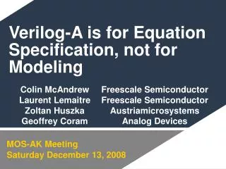
Verilog-A is for Equation Specification, not for Modeling. MOS-AK Meeting Saturday December 13, 2008. Overview. A Brief History of Verilog-A for Compact Modeling A Brief Review of How Circuit Simulators Work How to Leverage Understanding of How Simulators Work to Implement Desired Equations

E N D
Verilog-A is for Equation Specification, not for Modeling MOS-AK Meeting Saturday December 13, 2008
Overview • A Brief History of Verilog-A for Compact Modeling • A Brief Review of How Circuit Simulators Work • How to Leverage Understanding of How Simulators Work to Implement Desired Equations • thinking outside the “equivalent network” modeling box • example 1: BJT excess phase • example 2: single formulation resistor that can handle R=0 • Summary
What is Verilog-A? • Initially (mid to late 1990’s), a language for analog behavioral modeling to enable • top down AMS design at the block level • efficient top-level AMS verification • VHDL-AMS is a “competing” language developed around the same time for the same purposes • So how does Verilog-A relate to compact modeling?
Automation in Compact Modeling • In the late 1980’s automation began to creep into the development of simulators • especially for the time-consuming and error-prone task of implementing compact models (symbolic derivative generation) • added impetus to the on-going migration from “diffused” model code to “modular” model code • Simulator-model interfaces of the 1980’s and 1990’s: • WATAND • Saber/MAST – major commercial success • Tektronix (very early pioneer) • ADMIT plus various compilers (AT&T) • iSMILE • CMC Type-II interface (DOA circa 1995; engineering ≠ CS)
VBIC Eldo SP Spectre R3_CMC ADS Nexxim HiCUM BSIM aSPICE Mextram Nanosim PSP APLAC MM11 HSPICE EKV GoldenGate MOSVAR Ultrasim The Problem The Solution Common Language/Interface
Automated Model Implementation • Mostly flopped in mid 1990’s • VBIC was the first public model defined in high level code • generated FORTRAN and C also provided • these were used • high-level pseudo-code was not! (except by Tektronix) • chasm between engineers and advanced software techniques • Many misconceptions • code is slow compared to hand-coded C • within 10% of hand coded and getting better • will be faster one day (proven already), then works for all models! • cannot use for parameter extraction • if it’s in a simulator it’s in your simulator-based extractor! • different code for different simulators will give different results • different compile flags on the same platform give different results!
Enter Verilog-A • Significant issue with the concept (high-level language + compilers) was the lack of a standard high-level language! • Verilog-A was obviously the solution for this • VHDL-AMS touted as well initially • Minor deficiencies overcome by compact model additions defined in LRM2.2 • CMC accepted models defined in Verilog-A circa 2004 • Verilog-A has become the de facto standard language for defining compact models
Moving Beyond “Models” • You can use Verilog-A to define “physical” compact models • But this can be very restrictive • constrained to think in terms of equivalent networks • constrained to think in terms of I(V), Q(V) relations • A circuit simulator is an equation solver • Think of what equations you want to force the simulator to solve, then develop Verilog-A constructs to force this • not thinking in terms of physical representation
+ – How SPICE Works: Simple BJT Model and Circuit Ibc c Qbc Icc RB x b Vc Ibe Qbe Ib e RE
System Equations (DC): MNA • Unknowns are V(x), V(b), V(c), V(e), and Ic=I(Vc) x b e c • Vbe=V(b)–V(e) and Vbc=V(b) –V(c)
Branch Jacobian Entry (Element Matrix Stamp) • Solve KCL SI(V)=f(V)=0 at each node, plus the “voltage equation” for voltage sources (and inductors) • nonlinear, so need iterative Newton solution • Vk+1=Vk+dVk, JkdVk=-f(Vk), Jk= ∂I/∂V|V=Vk • Easy to set up Jacobian Jk in an algorithmic fashion • rows are defined by nodes that the current flows between • +ve for flow into node, –ve for flow out-of node • columns are defined by the branch control voltages • +ve for first node, –ve for second, for Vab=V (a)-V (b) • voltage sources and inductors add a row for the voltage equation and a column (unknown system variable) for the current
V(x) V(b) V(c) V(e) Ic SI(x) SI(b) SI(c) SI(e) Vc Jacobian Assembly (“Stamping”) • gbe=∂Ibe/Vbe • gce=∂Icc/Vbe, gcc=∂Icc/Vbc,gm= gce+ gcc , go= - gcc
SPICE • Circuit simulators are not really “circuit simulators” • for DC they are multidimensional nonlinear equation solvers • for transient they are nonlinear ordinary differential equation (ODE) solvers • multidimensional nonlinear equation solvers at each time point • Instead of thinking of Verilog-A as a means to define equivalent network models, think of it as a means of specifying equations for numerical solution • formulate the equations you want • understand how MNA equations are set up • work out how to use Verilog-A to set up the desired equations
Itxf =V(xf2) TD/3 xf1 xf2 Itzf TD 1W Weil-McNamee Excess Phase for BJTs • Goal: implement a phase shift for gm with the least possible change in the magnitude of gm • network approach leads to 2nd order Bessel (linear phase) filter • straight forward to implement as RLC circuit (L. Wagner, IBM)
xf2 xf1 Itzf V(xf2) V(xf1) TD TD/3 1W How Can We Get Rid of the Pesky Inductor?
Itxf =2V(xf)- Itzf xf Itzf TD/2 1W Can We Better Approximate an Ideal Phase Shift? • Only 1 added system variable!
The “Solution” ... sort of • For “reasonable” R: • natural for NA (SPICE) • efficient for NA • nasty for R=0 or small R • For “small” R: • extra MNA system variable • no worries for R=0 or small R
The “... sort of” Solution `include "disciplines.h" `define rm 0.001 module r_va(p,m); inout p,m; electrical p,m; parameter real R = 1.0 from[0.0:inf); analog begin : analogBlock if (R<`rm) V(p,m) <+ I(p,m)*R; else I(p,m) <+ V(p,m)/R; end // analogBlock endmodule EASY TO DEFINE HARD TO IMPLEMENT
Why “... sort of” is not Enough • Does work in Verilog-A • excellent feature of the language • Does not (easily) work for • built-in model implementation via ADMS • some model interfaces for some simulators • dynamic switching for the case when R varies with bias • Do not want to switch formulations during iterative solution • dynamically adds extra system variable I(p,m) • Observation: must have this current for V=RI formulation • Conclusion: explicitly include in model formulation
V(p) V(m) I_r V(p,m) How do We Force Verilog-A to do What We Want? • For simplicity of implementation in model interfaces, need to get rid of voltage contribution • only want strict nodal analysis formulation • How can we do this for R=0? • Want V(p,m)=0 • Set up currentcontribution forthis as the only flowinto a node • Forces set up ofequation we want!
The R=0 Solution `include "disciplines.h" module r_va(p,m); inout p,m; electrical p,m,I_r; parameter real R = 1.0 from[0.0:inf); analog begin : analogBlock I(I_r) <+ V(p,m); I(p,m) <+ 1.0e-6*V(I_r); end // analogBlock endmodule second equation forces V(I_r) to be current flowing between p and m
Extension for Small Nonzero R `include "disciplines.h" module r_va(p,m); inout p,m; electrical p,m,I_r; parameter real R = 1.0 from[0.0:inf); analog begin : analogBlock I(I_r) <+ V(p,m)-1.0e-6*R*V(I_r); I(p,m) <+ 1.0e-6*V(I_r); end // analogBlock endmodule first equation forces V(p,m)=I*R (voltage on node I_r is current p→m)
Final Result `include "disciplines.h" `define rm 0.001 module r_va(p,m); inout p,m; electrical p,m,I_r; parameter real R = 1.0 from[0.0:inf); analog begin : analogBlock I(I_r) <+ V(p,m)-1.0e-6*R*V(I_r); if (R<`rm) I(p,m) <+ 1.0e-6*V(I_r); else I(p,m) <+ V(p,m)/R; // I=G*V formulation end // analogBlock endmodule
Final Model • Manipulated Verilog-A equations we want to solve • Resistor model that does not switch formulations from current contribution to voltage contribution • strictly nodal formulation • easy to implement in all simulator model interfaces • numerically well behaved for all R≥0 • can be adapted to use same “switch” for voltage variable R • direct bias dependence • indirect bias dependence (e.g. self-heating) • Cost is added system variable V(I_r) is added for all values of R, not just R<`rm
Summary • Circuit simulators are equation, not circuit, solvers • Historical modeling approach of equivalent networks and a physical approach may not always give desired result • By thinking about what equations you want to implement or solve, and understanding how MNA is set up, you can use Verilog-A to implement “non-obvious” but useful models • Note: if “currents” are mapped to node voltages (i.e. system variables), they need to be scaled by the voltage/current tolerance ratio (default is 1.0e6)